The tutorial shows how to safely merge rows in Excel in 4 different ways: merge multiple rows without losing data, combine duplicate rows, repeatedly merge blocks of rows, and copy matching rows from another table based on one or more common columns.
Merging rows in Excel is one of the most common tasks that all of us need to perform every now and then. The problem is that Microsoft Excel does not provide a reliable tool to do this. For example, if you try to combine two or more rows using the built-in Merge & Center button, you will end up with the following error message:
"The selection contains multiple data values. Merging into one cell will keep the upper-left most data only."

Clicking OK will merge the cells but only keep the value of the first cell, all other data will be gone. So, obviously we need a better solution. This article describes several methods that will let you merge multiple rows in Excel without losing any data.
How to merge rows in Excel without losing data
The task: you have a database where each row contains certain details such as product name, product key, customer name and so on. What we want is to combine all the rows related to a particular order like shown below:
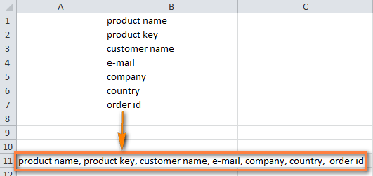
There are two ways to achieve the desired result:
Merge multiple rows using formulas
To joint the values from several cells into one, you can use either the CONCATENATE function or concatenation operator (&). In Excel 2016 and higher, you can also use the CONCAT function. Any way, you supply cells as references and type the desired delimiters in-between.
Merge rows and separate the values with comma and space:
=CONCATENATE(A1,", ",A2,", ",A3)
=A1&", "&A2&", "&A3
Merge rows with spaces between the data:
=CONCATENATE(A1," ",A2," ",A3)
=A1&" "&A2&" "&A3
Combine rows and separate the values with commas without spaces:
=CONCATENATE(A1,A2,A3)
=A1&","&A2&","&A3
In practice, you may often need to concatenate more cells, so your real-life formula is likely to be a bit longer:
=CONCATENATE(A1,", ",A2,", ",A3,", ",A4,", ",A5,", ",A6,", ",A7,", ",A8)
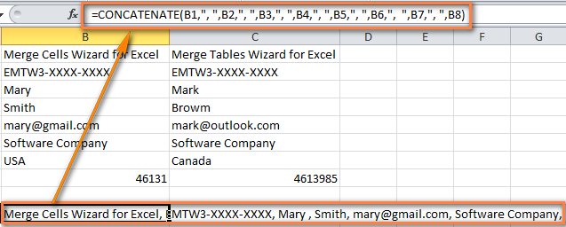
Now you have several rows of data merged into one row. But your combined rows are formulas. To convert them to values, use the Paste Special feature as described in How to replace formulas with their values in Excel.
Combine rows in Excel with Merge Cells add-in
The Merge Cells add-in is a multi-purpose tool for joining cells in Excel that can merge individual cells as well as entire rows or columns. And most importantly, this tool keeps all the data even if the selection contains multiple values.
To merge two or more rows into one, here's what you need to do:
- Select the range of cells where you want to merge rows.
- Go to the Ablebits Data tab > Merge group, click the Merge Cells arrow, and then click Merge Rows into One.

- This will open the Merge Cells dialog box with the preselected settings that work fine in most cases. In this example, we only change the separator from the default space to line break, as shown in the screenshot below:

- Click the Merge button and observe the perfectly merged rows of data separated with line breaks:

How to combine duplicate rows into one (keeping unique values only)
The task: you have some Excel database with a few thousand entries. The values in one column are essentially the same while data in other columns are different. Your goal is to combine data from duplicate rows based on a certain column, making a comma separated list. Additionally, you may want to merge unique values only, omitting duplicates and skipping empty cells.
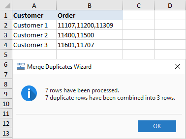
The screenshot below shows what we are trying to achieve.
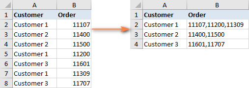
The prospect of finding and merging duplicate rows manually is definitely something you'd want to avoid. Meet the Merge Duplicates add-in that turns this time-consuming and cumbersome chore into a quick 4-steps process.
- Select the duplicate rows you want to merge and run the Merge Duplicates wizard by clicking its button on the ribbon.

- Make sure your table is selected correctly and click Next. It is wise to keep the Create a backup copy option checked, especially if you are using the add-in for the first time.
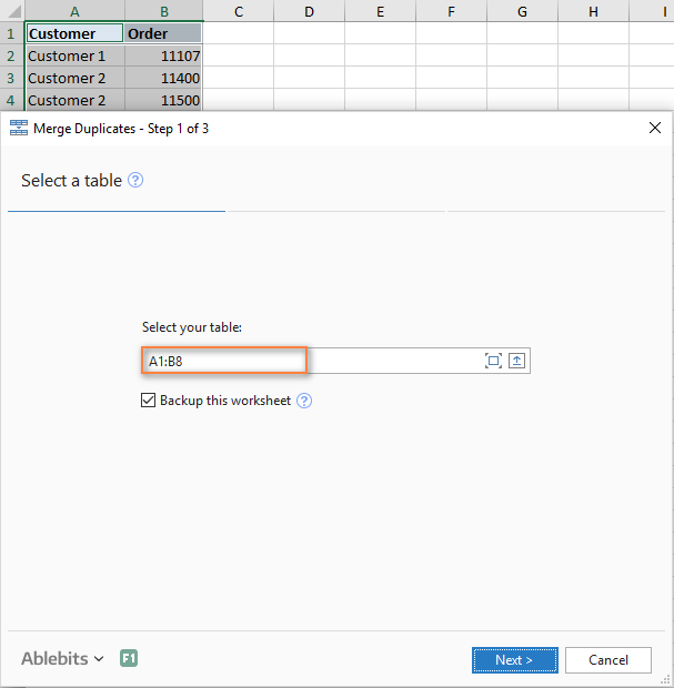
- Select the key column to check for duplicates. In this example, we select the Customer column because we want to combine rows based on customer name.
If you want to skip empty cells, be sure to select this option and click Next.

- Choose the columns to merge. In this step, you select the columns whose data you want to combine data and specify the delimiter: semicolon, comma, space, line break, etc.
Two additional options in the upper part of the window let you:
- Delete duplicate values while combining the rows
- Skip empty cells
When done, click the Finish button.

In a moment, all the data from duplicate rows are merged into one row:
How to repeatedly merge blocks of rows into one row
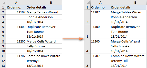
The task: you have an Excel file with information about the recent orders and each order takes 3 lines: product name, customer name and date of purchase. You would like to merge every three rows into one, i.e. repeatedly merge the blocks of three rows.
The following image show what we are looking for:
If there are only few entries to be combined, you can select each 3 rows and merge each block individually using the Merge Cells add-in. But if your worksheet contains hundreds or thousands of records, you will need a faster way:
- Add a helper column to your worksheet, column C in our example. Let's name it BlockID, or whatever name you like.
- Insert the following formula in C2 and then copy it down the column by dragging the fill handle:
=INT((ROW(C2)-2)/3)Where:
- C2 is the topmost cell in which you enter the formula
- 2 is the row where the data starts
- 3 is the number of rows to be combined in each block
This formula adds a unique number to each block of rows, as shown in the screenshot:

How this formula works: The ROW function extracts the row number of the formula cell, from which you subtract the number of the row where your data start, so that the formula starts counting from zero. For example, our data start in the 2nd row, so we subtract 2. If your data start, say, in row 5, then you will have ROW(C5)-5. After that, you divide the above equation by the number of rows to be merged and use the INT function to round the result down to the nearest integer. - Well, you've done the main part of the work. Now you just need to merge the rows based on the BlockID For this, we will be using the already familiar Merge Duplicates wizard that we utilized for combining duplicate rows:
- In step 2, choose BlockID as the key column.
- In step 3, select all the columns you want to merge and pick line break as the delimiter.

In a moment, you will have the desired result:

- Delete the Block ID column since you don't need it any longer and you are done! A funny thing is that we've needed 4 steps again, like in the two previous examples :)
How to merge matching rows from 2 Excel tables without copying / pasting
Task: you have two tables with a common column(s) and you need to merge matching rows from those two tables. The tables may be located in the same sheet, in two different spreadsheets or in two different workbooks.
For example, we have sales reports for January and February in two different worksheets and want to combine them into one. Mind you, each table may have a different number of rows and different order of products, therefore simple copy/pasting won't work.
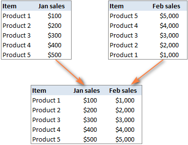
In this case, the Merge Two Tables add-in will work a treat:
- Select any cell in your main table and click the Merge Two Tables button on the Ablebits Data tab, in the Merge group:

This will run the add-in with your main table preselected, so in the first step of the wizard you simply click Next. - Select the second table, i.e. the lookup table containing the matching rows.

- Choose one or more column columns that exist in both tables. The key columns should contain only unique values, like Product ID in our example.

- Optionally, select the columns to update in the main table. In our case, there are no such columns, so we just click Next.
- Choose the columns to add to the main table, Feb sales in our case.

- In the final step, you can select additional options depending on how exactly you want to merge data, and click the Finish button. The screenshot below shows the default settings, that work just fine for us:

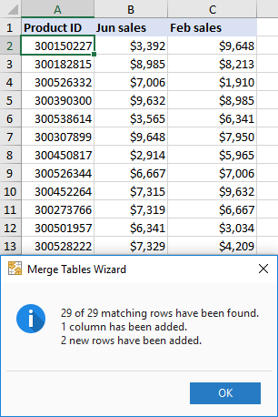
Allow the add-in a few seconds for processing and review the result:
How can I get these merging tools for Excel?
All of the add-ins discussed in this tutorial, plus 70+ other time-saving tools, are included in our Ultimate Suite for Excel. The add-ins work with all versions of Excel 2019, Excel 2016, Excel 2013, Excel 2010 and Excel 2007.
Hopefully, you can now merge rows in your Excel sheets exactly the way you want them. If you have not found a solution for your specific task, just leave a comment and we will try to figure out a way together. Thank you for reading!
Available downloads
Ultimate Suite 14-day fully-functional version (.exe file)
 by
by
26 comments
Goodday
question; i have an excel spreadsheet with daily sales of three mths and nine stores ,i will like to place this document into one sheet for nine stores so i can be able to see what what the stores sold by week.
Hi! Depending on what you want to do, there may be different answers. Try using a pivot table to show data for any store for any period of time. You can also use the FILTER function to get sales data by store for a week. To simply calculate the sum of sales for the week, you can use the SUMIFS function.
I have the following group of data in excel:
Location
ID
Name
Grade
Subject
Cred Term
Doc #
Eff Beg
Eff end
Some ID's have multiple lines as they have multiple certifications. I would like to merge all certifications into one line by ID.
I currently have Ablebits software.
Hi!
Use Ablebits Data - Merge Duplicates.
Step 1. Select your table.
Step 2. Choose key columns - select ID column
Step 3. Choose columns with the values to merge - select all other cloumns or only some of the columns whose data needs to be merged
You can also read the detailed instructions for the Merge Duplicates tool here: How to combine duplicate rows in Excel.
I hope I answered your question. If something is still unclear, please feel free to ask.
Hi!! Thank you for helping people find solutions! How do I merge duplicate rows (of customers) info into one row with the customers info in multiple columns?
Like Customer one came into the store on dates (data in each row in separate columns) so each customer only has 1 row instead of 5 rows.
My end goal is to have Customer 1 in one row with all of their visit dates in one row. Right now, there Visit dates are on their own row (but in different columns).
Thx!!
Kelley
Hello!
I recommend that you use the Merge Duplicates tool. You can quickly combine duplicate rows into one without losing any data. It is available as a part of our Ultimate Suite for Excel that you can install in a trial mode and check how it works for free.
Hi. re: "How to combine duplicate rows into one (keeping unique values only)" section of this article, does Ablebits have a tool that will do the inverse/opposite of this? i.e. delimit the merged values and repeat/duplicate the respective key column value for each of the delimited values?
To elaborate a little more, what I am trying to achieve is similar to what is described here:
http s://stackoverflow.com/questions/44655553/vba-excel-with-thousands-of-rows-how-to-transpose-variable-length-columns-to
But instead of a macro, I am wondering if Ablebits offers a tool that does the same?
Hello!
We have a tool that can solve your task in a couple of clicks - first you use the tool Merge Cells - Merge Columns Into One. You are merge the Property1-Property6 values in one column by separating them with a semicolon, for example. Then you use Split Text - Split by Characters - Split to Rows and get the desired result.
It is available as a part of our Ultimate Suite for Excel that you can install in a trial mode and check how it works for free.
Hello!
You can get all the unique values in one cell using the Duplicate Remover - Uniques and 1st Occurrences tools.
You can split these values into cells using the Split Text tool.
However, Ultimate Suite cannot restore the previous number of duplicates and return data to its original state.
You can install Ultimate Suite for Excel in a trial mode and check how it works for free.
is there a short way l could merge rows with even gaps into one row. l am using a sheet with several line items which have different row gaps.
Hello,
the simplest and quickest way of combining the rows is using our add-ins: Merge Cells and Combine Rows Wizard.
You can see how they work in the article above and you can also download and install their fully-functional versions to try them out.
Dear Irina,
I need to merge multiple rows in the same column with one another so that you have all text in one column, and row. Can you please help?
Kind regards
Jan Swart
Dear Jan,
we have just a perfect solution for you - Merge Cells Wizard. With its help, you'll be able to combine multiple cells into one cell/row/column and use any separator to your liking.
You can download and install the trial version of the add-in by using this direct link.
Please find the instructions on how to work with the add-in on its help page.
Hope you'll find the add-in useful!
Irina,
I have two rows, 3 columns with Col A Name, Col B expiration date and Col C email address.
Row 1has the name and email address
Row 2 has the name and expiration date
I need to merge, combine, sort; to obtain the name, expiration date and email address into one row of data
Example:
row 1 Fred fred@fred
row 2 Fred 12/1/2017
Need row Fred 12/1/2017 fred@fred
Hi Charles,
You can use our Combine Rows Wizard add-in to solve this task:
https://www.ablebits.com/excel-combine-rows/index.php
I have a list of contacts to merge. Some rows are for the same person, and have different data than the other rows. One may have an email address, the other the phone number. Sometimes both rows have the same data.
The prior comments are all interesting, but did not have this answer.
Is there a way to merge the rows and retain the best data? I would think I need a VBA macro which allows a dialog box for me to choose the better of the two data points if there is competing data for a column.
This may not be a strictly Excel solution, but do you have any advice for this very common scenario?
Thank you
Hello Curt,
Combine Rows Wizard does exactly what you describe:
https://www.ablebits.com/excel-combine-rows/index.php
You can specify the key columns to know the rows refer to the same record, like the name, and select all other columns for the merge with the option to delete duplicate values; thus you'll get all relevant information on the same row.
Hi,
Is there a way to use the combine rows and have the program actually write out all the columns instead of entering data in a column separated by semicolons or commas? I want the duplicate data actually expanded across columns:
Sample
A B 32 25 Y N
A C 32 22 N Y
Combined
A B C 32 32 35 22 Y N N Y
I love the program, it is fantastic but I need to expand the results and not sure how to do that.
Thanks,
Gene
Hello Gene,
If you have simple data (without commas), the following solution might work for you:
1 Run Combine Rows Wizard to merge the data and choose a semicolon as the separator.
2 Save the resulting worksheet as a .csv file. For more details, please see this article:
https://www.ablebits.com/office-addins-blog/convert-excel-csv/
3 Open the .csv file in Notepad and replace all semicolons with commas. Save the file.
4 Open the .csv file in Excel, see here for full details:
https://www.ablebits.com/office-addins-blog/convert-csv-excel/
I am having a 5000 customer in Column "A" and In column "A' most of the customer is repeated Now i want the formulas from which i will check the names of the customer which is present in this column.
Hello John,
There exist a number of solutions depending on what exactly result you are trying to achieve.
If you want to highlight all duplicates in a column, please see this article:
https://www.ablebits.com/office-addins-blog/how-to-highlight-duplicates-excel/
To highlight duplicate entries between 2 columns, see the "Compare 2 columns for duplicates" example on this page:
https://www.ablebits.com/office-addins-blog/excel-conditional-formatting-formulas/
If you want to merge the duplicate rows into one, check out the Combine Duplicated Rows add-in:
https://www.ablebits.com/excel-combine-rows/index.php
let's say I have 2 rows of the exact same data, except for ONE cell in each column.
For an example, let's make the headers: a. Customer Name, b. Customer ID, c. Customer Address, and d. Amount Paid.
Now rows 1 & 2 are the exact same customer, except in row 1 column d the dollar amount is $500, and in row 2 the dollar amount is $300.
Is there a way to quickly consolidate into a single line, with the dollar amount in column d the sum of the previous entries? (i.e. $800)?
Hello Harold,
You can do this in 2 ways:
1. Using Subtotal. Sort your table by Customer ID and then apply subtotal in this way: At each change in "Customer ID", use function "Sum", add subtotal to column "Amount Paid". Please see this article for more details: Using Subtotals in Microsoft Excel
2. Using a pivot table.
Hey Friend If u are still here so please tell me how to Merge or combine two column without losing data...like 1 have numbers in A1 and AW1,AX1 both had merged.i want copy A1 number to AW1,AX1...i Have a Very Big Spreadsheet..is it Possible or i ahve to do Manually...please Reply Fast..Thanks...
Hi Akbar,
You can find several solutions in this article: How to merge two columns in Excel without losing data. Hope you will find them helpful.