These examples will teach you how to Vlookup multiple criteria, return a specific instance or all matches, do dynamic Vlookup in multiple sheets, and more.
It is the second part of the series that will help you harness the power of Excel VLOOKUP. The examples imply that you know how this function works. If not, it stands to reason to start with the basic uses of VLOOKUP in Excel.
Before moving further, let me briefly remind you the syntax:
Now that everyone is on the same page, let's take a closer look at the advanced VLOOKUP formula examples:
How to Vlookup multiple criteria
The Excel VLOOKUP function is really helpful when it comes to searching across a database for a certain value. However, it lacks an important feature - its syntax allows for just one lookup value. But what if you want to look up with several conditions? There are a few different solutions for you to choose from.
Formula 1. VLOOKUP with two criteria
Suppose you have a list of orders and want to find the quantity based on 2 criteria, Customer name and Product. A complicating factor is that each customer ordered multiple products, as shown in the table below:
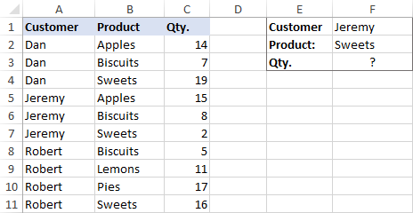
A usual VLOOKUP formula won't work in this situation because it returns the first found match based on a single lookup value that you specify.
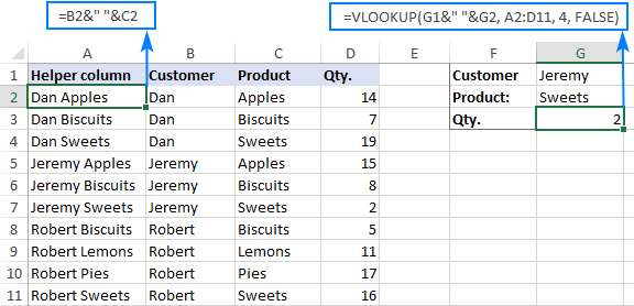
To overcome this, you can add a helper column and concatenate the values from two lookup columns (Customer and Product) there. It is important that the helper column should be the leftmost column in the table array because it's where Excel VLOOKUP always searches for the lookup value.
So, add a column to the left of your table and copy the below formula across that column. This will populate the helper column with the values from columns B and C (the space character is concatenated in between for better readability):
=B2&" "&C2
And then, use a standard VLOOKUP formula and place both criteria in the lookup_value argument, separated with a space:
=VLOOKUP("Jeremy Sweets", A2:D11, 4, FALSE)
Or, input the criteria in separate cells (G1 and G2 in our case) and concatenate those cells:
=VLOOKUP(G1&" "&G2, A2:D11, 4, FALSE)
As we want to return a value from column D, which is fourth in the table array, we use 4 for col_index_num. The range_lookup argument is set to FALSE to Vlookup an exact match. The screenshot below shows the result:
In case your lookup table is in another sheet, include the sheet's name in your VLOOKUP formula. For example:
=VLOOKUP(G1&" "&G2, Orders!A2:D11, 4, FALSE)
Alternatively, create a named range for the lookup table (say, Orders) to make the formula easier-to-read:
=VLOOKUP(G1&" "&G2, Orders, 4, FALSE)
For more information, please see How to Vlookup from another sheet in Excel.
Note. For the formula to work correctly, the values in the helper column should be concatenated exactly the same way as in the lookup_value argument. For example, we used a space character to separate the criteria in both the helper column (B2&" "&C2) and VLOOKUP formula (G1&" "&G2).
Formula 2. Excel VLOOKUP with multiple conditions
In theory, you can use the above approach to Vlookup more than two criteria. However, there are a couple of caveats. Firstly, a lookup value is limited to 255 characters, and secondly, the worksheet's design may not allow adding a helper column.
Luckily, Microsoft Excel often provides more than one way to do the same thing. To Vlookup multiple criteria, you can use either an INDEX MATCH combination or the XLOOKUP function recently introduced in Office 365.
For example, to look up based on 3 different values (Date, Customer name and Product), use one of the following formulas:
=INDEX(D2:D11, MATCH(1, (G1=A2:A11) * (G2=B2:B11) * (G3=C2:C11), 0))
=XLOOKUP(1, (G1=A2:A11) * (G2=B2:B11) * (G3=C2:C11), D2:D11)
Where:
- G1 is criteria 1 (date)
- G2 is criteria 2 (customer name)
- G3 is criteria 3 (product)
- A2:A11 is lookup range 1 (dates)
- B2:B11 is lookup range 2 (customer names)
- C2:C11 is lookup range 3 (products)
- D2:D11 is the return range (quantity)
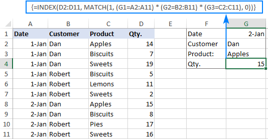
Note. In all versions except Excel 365, INDEX MATCH should be entered as an CSE array formula by pressing Ctrl + Shift + Enter. In Excel 365 that supports dynamic arrays it also works as a regular formula.
For the detailed explanation of the formulas, please see:
How to use VLOOKUP to get 2nd, 3rd or nth match
As you already know, Excel VLOOKUP can fetch only one matching value, more precisely, it returns the first found match. But what if there are several matches in your lookup array and you want to get the 2nd or 3rd instance? The task sounds quite intricate, but the solution does exist!
Formula 1. Vlookup Nth instance
Suppose you have customer names in one column, the products they purchased in another, and you are looking to find the 2nd or 3rd product bought by a given customer.
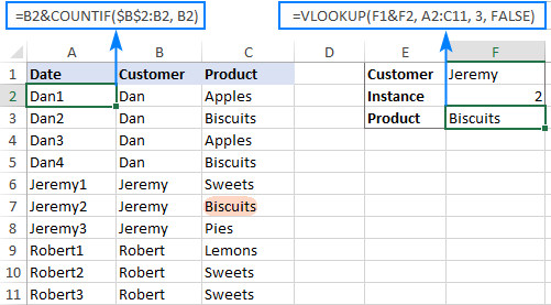
The simplest way is to add a helper column to the left of the table like we did in the first example. But this time, we will populate it with customer names and occurrence numbers like "John Doe1", "John Doe2", etc.
To get the occurrence, use the COUNTIF function with a mixed range reference (the first reference is absolute and the second is relative like $B$2:B2). Since the relative reference changes based on a position of the cell where the formula is copied, in row 3 it will become $B$2:B3, in row 4 - $B$2:B4, and so on.
Concatenated with the customer name (B2), the formula takes this form:
=B2&COUNTIF($B$2:B2, B2)
The above formula goes to A2, and then you copy it down to as many cells as needed.
After that, input the target name and occurrence number in separate cells (F1 and F2), and use the below formula to Vlookup a specific occurrence:
=VLOOKUP(F1&F2, A2:C11, 3, FALSE)
Formula 2. Vlookup 2nd occurrence
If you are looking for the 2nd instance of the lookup value, then you can do without the helper column. Instead, create the table array dynamically by using the INDIRECT function together with MATCH:
=VLOOKUP(E1, INDIRECT("A"&(MATCH(E1, A2:A11, 0)+2)&":B11"), 2, FALSE)
Where:
- E1 is the lookup value
- A2:A11 is the lookup range
- B11 is the last (bottom-right) cell of the lookup table

Please note that the above formula is written for a specific case where data cells in the lookup table begin in row 2. If your table is somewhere in the middle of the sheet, use this universal formula, where A1 is the top-left cell of the lookup table containing a column header:
=VLOOKUP(E1, INDIRECT("A"&(MATCH(E1, A2:A11, 0)+1+ROW(A1))&":B11"), 2, FALSE)
How this formula works
Here is the key part of the formula that creates a dynamic vlookup range:
INDIRECT("A"&(MATCH(E1, A2:A11, 0)+2)&":B11")
The MATCH function configured for exact match (0 in the last argument) compares the target name (E1) against the list of names (A2:A11) and returns the position of the first found match, which is 3 in our case. This number is going to be used as the starting row coordinate for the vlookup range, so we add 2 to it (+1 to exclude the first instance and +1 to exclude row 1 with the column headers). Alternatively, you can use 1+ROW(A1) to calculate the necessary adjustment automatically based on the position of the header row (A1 in our case).
As the result, we get the following text string, which INDIRECT converts to a range reference:
INDIRECT("A"&5&":B11") -> A5:B11
This range goes to the table_array argument of VLOOKUP forcing it to start searching in row 5, leaving out the first instance of the lookup value:
VLOOKUP(E1, A5:B11, 2, FALSE)
How to Vlookup and return multiple values in Excel
The Excel VLOOKUP function is designed to return just one match. Is there a way to Vlookup multiple instances? Yes, there is, though not an easy one. This requires a combined use of several functions such as INDEX, SMALL and ROW is an array formula.
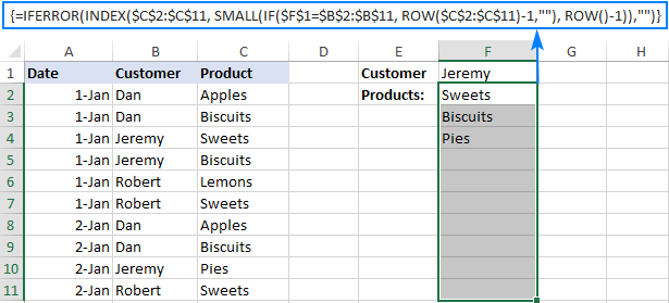
For example, the below can find all occurrences of the lookup value F2 in the lookup range B2:B16 and return multiple matches from column C:
{=IFERROR(INDEX($C$2:$C$11, SMALL(IF($F$1=$B$2:$B$11, ROW($C$2:$C$11)-1,""), ROW()-1)),"")}
There are 2 ways to enter the formula in your worksheet:
- Type the formula in the first cell, press Ctrl + Shift + Enter, and then drag it down to a few more cells.
- Select several adjacent cells in a single column (F1:F11 in the screenshot below), type the formula and press Ctrl + Shift + Enter to complete it.
Either way, the number of cells in which you enter the formula should be equal to or larger than the maximum number of possible matches.
For the detailed explanation of the formula logic and more examples, please see How to VLOOKUP multiple values in Excel.
How to Vlookup in rows and columns (two-way lookup)
Two-way lookup (aka matrix lookup or 2-dimentional lookup) is a fancy word for looking up a value at the intersection of a certain row and column. There are a few different ways to do two-dimensional lookup in Excel, but since the focus of this tutorial is on the VLOOKUP function, we will naturally use it.
For this example, we'll take the below table with monthly sales and work out a VLOOKUP formula to retrieve the sales figure for a specific item in a given month.
With item names in A2:A9, month names in B1:F1, the target item in I1 and the target month in I2, the formula goes as follows:
=VLOOKUP(I1, A2:F9, MATCH(I2, A1:F1, 0), FALSE)

How this formula works
The core of the formula is the standard VLOOKUP function that searches for an exact match to the lookup value in I1. But since we do not know in which exactly column the sales for a specific month are, we cannot supply the column number directly to the col_index_num argument. To find that column, we use the following MATCH function:
MATCH(I2, A1:F1, 0)
Translated into English, the formula says: look up the I2 value in A1:F1 and return its relative position in the array. By supplying 0 to the 3rd argument, you instruct MATCH to find the value exactly equal to the lookup value (it's like using FALSE for the range_lookup argument of VLOOKUP).
Since Mar is in the 4th column in the lookup array, the MATCH function returns 4, which goes directly to the col_index_num argument of VLOOKUP:
VLOOKUP(I1, A2:F9, 4, FALSE)
Please pay attention that although the month names start in column B, we use A1:I1 for the lookup array. This is done in order for the number returned by MATCH to correspond to the column's position in table_array of VLOOKUP.
To learn more ways to perform matrix lookup in Excel, please see INDEX MATCH MATCH and other formulas for 2-dimensional lookup.
How to do multiple Vlookup in Excel (nested Vlookup)
Sometimes it may happen that your main table and lookup table do not have a single column in common, which prevents you from doing a Vlookup between two tables. However, there exists another table, which does not contain the information you are looking for but has one common column with the main table and another common column with the lookup table.
In below image illustrates the situation:
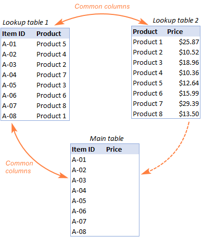
The goal is to copy prices to the main table based on Item IDs. The problem is that the table containing prices does not have the Item IDs, meaning we will have to do two Vlookups in one formula.
For the sake of convenience, let's create a couple of named ranges first:
- Lookup table 1 is named Products (D3:E10)
- Lookup table 2 is named Prices (G3:H10)
The tables can be in the same or different worksheets.
And now, we will perform the so-called double Vlookup, aka nested Vlookup.
First, make a VLOOKUP formula to find the product name in the Lookup table 1 (named Products) based on the item id (A3):
=VLOOKUP(A3, Products, 2, FALSE)
Next, put the above formula in the lookup_value argument of another VLOOKUP function to pull prices from Lookup table 2 (named Prices) based on the product name returned by the nested VLOOKUP:
=VLOOKUP(VLOOKUP(A3, Products, 2, FALSE), Prices, 2, FALSE)
The screenshot below shows our nested Vlookup formula in action:

How to Vlookup multiple sheets dynamically
Sometimes, you may have data in the same format split over several worksheets. And your aim is to pull data from a specific sheet depending on the key value in a given cell.
This may be easier to understand from an example. Let's say, you have a few regional sales reports in the same format, and you are looking to get the sales figures for a specific product in certain regions:

Like in the previous example, we start with defining a few names:
- Range A2:B5 in CA sheet is named CA_Sales.
- Range A2:B5 in FL sheet is named FL_Sales.
- Range A2:B5 in KS sheet is named KS_Sales.
As you can see, all the named ranges have a common part (Sales) and unique parts (CA, FL, KS). Please be sure to name your ranges in a similar manner as it's essential for the formula we are going to build.
Formula 1. INDIRECT VLOOKUP to dynamically pull data from different sheets
If your task is to retrieve data from multiple sheets, a VLOOKUP INDIRECT formula is the best solution – compact and easy-to-understand.
For this example, we organize the summary table in this way:
- Input the products of interest in A2 and A3. Those are our lookup values.
- Enter the unique parts of the named ranges in B1, C1 and D1.
And now, we concatenate the cell containing the unique part (B1) with the common part ("_Sales"), and feed the resulting string to INDIRECT:
INDIRECT(B$1&"_Sales")
The INDIRECT function transforms the string into a name that Excel can understand, and you put it in the table_array argument of VLOOKUP:
=VLOOKUP($A2, INDIRECT(B$1&"_Sales"), 2, FALSE)
The above formula goes to B2, and then you copy it down and to the right.
Please pay attention that, in the lookup value ($A2), we've locked the column coordinate with absolute cell reference so that the column remains fixed when the formula is copied to the right. In the B$1 reference, we locked the row because we want the column coordinate to change and supply an appropriate name part to INDIRECT depending on the column into which the formula is copied:

If your main table is organized differently, the lookup values in a row and unique parts of the range names in a column, then you should lock the row coordinate in the lookup value (B$1) and the column coordinate in the name parts ($A2):
=VLOOKUP(B$1, INDIRECT($A2&"_Sales"), 2, FALSE)

Formula 2. VLOOKUP and nested IFs to look up multiple sheets
In situation when you have just two or three lookup sheets, you can use a fairly simple VLOOKUP formula with nested IF functions to select the correct sheet based on the key value in a particular cell:
=VLOOKUP($A2, IF(B$1="CA", CA_Sales, IF(B$1="FL", FL_Sales, IF(B$1="KS", KS_Sales,""))), 2, FALSE)
Where $A2 is the lookup value (item name) and B$1 is the key value (state):

In this case, you do not necessarily need to define names and can use external references to refer to another sheet or workbook.
For more formula examples, please see How to VLOOKUP across multiple sheets in Excel.
That's how to use VLOOKUP in Excel. I thank you for reading and hope to see you on our blog next week!
Practice workbook for download
Advanced VLOOKUP formula examples (.xlsx file)
 by
by
540 comments
I want to transfer data from one excel sheet to another in the same work book. Hence the code =VLOOKUP(I4&B8,info!A6:J335,4,0). How do i anchor this code.
Thanks.
Hello Elijah!
I don't have your data, so try using these recommendations: How to VLOOKUP between two sheets.
Good Day: How would one use multi factor lookup with numeric data specifically where the second criteria would use the range_lookup=True to find something in between values in the second column. Example below.
Using the table below, criteria provided would be year (e.g. 2025) and Amount (e.g. 120). Desired return 2025, 120 would be 21.0% for col 3 return and $2100 for col 4 return
Year Amount Pct Payment
2024 0 10% $1,000
2024 100 20% $2,000
2024 200 30% $3,000
2024 300 40% $4,000
2025 0 10.5% $1,050
2025 115 21.0% $2,100
2025 230 31.5% $3,150
2025 345 42.0% $4,200
2026 0 11.0% $1,103
2026 132. 22.1% $2,205
2026 264 33.1% $3,308
2026 396 44.1% $4,410
2027 0 11.6% $1,158
2027 152 23.2% $2,315
2027 304 34.7% $3,473
2027 456 46.3% $4,631
Thanks in advance: Dan
Hi! You can use INDEX MATCH to search for a value based on two conditions. For the detailed instructions, please see: Excel INDEX MATCH with multiple criteria - formula examples.
=INDEX(C2:C20,MATCH($F$1,B2:B20/(A2:A20=$E$1),1))
F1 = 120. E1 = 2025.
For MATCH function, use the approximate search as described in this manual: How to use MATCH function in Excel. This should solve your task.
Thanks for your reply. Your suggested formula returns #VALUE!. My exact formula is below (I modified my sheet to match your inputs and the range of the data)
=INDEX(C2:C17,MATCH($F$1,B2:B17/(A2:A17=$E$1),1))
Double clicking the formula highlights the correct ranges and criteria cells.
When doing Evaluate Formula, ranges B2:B17 and A2:A17 both evaluate to #VALUE! (in that order). Both F1 and E1 come in properly.
What am I missing?
Hi! The formula I sent to you was created based on the description you provided in your first request. The formula works correctly with this data. Check your data.
Nevermind: I just caught that this should be an Array type of formula (CTRL-SHIFT-ENTER).
Thanks
I am currently using VLOOKUP to return a value from one sheet to another.
=VLOOKUP(C9,Rates!$B$3:$C$57,2,0)
I would like to add additional conditions to this formula so that it will look up the value in C9 and then E9 to return the value of the corresponding cell on the Rates sheet.
B C D E
3 POSITION ST OT DT
5 MANAGER 172 220 294
6 SUPERVISOR 169 217 290
if vlookup finds Manager (B5) and ST (C3), it will return 172 (C5), Manager (B5) and DT (E3) will return 294 (E5), Supervisor (B6) and OT (D3) will return 217 (D6)
should I use IFS or IFSERROR?
Hello Dawn!
Pay attention to the following paragraph of the article above: How to Vlookup multiple criteria.
You can also find useful information in this article: Excel INDEX MATCH with multiple criteria.
You can also use the XLOOKUP formula. Read more: XLOOKUP with multiple criteria.
In situations where you need to perform multiple Vlookups based on the success or failure of the previous Vlookup, you can nest two or more IFERROR functions. For more information, please visit: Nested IFERROR functions to do sequential Vlookups in Excel.
Which Excel formula should I use to have the number of actions from the first column (OWNER) that are closed (COLUMN 8 (STATUS Open / In Progress / Closed)
In the First column you will have different B numbers (B01, B02, B03, B04, etc.)
Hello Carlos! If I understand your task correctly, this guide may be helpful: COUNTIF with wildcard characters (partial match). Please check the formula below, it should work for you:
=COUNTIF(A2:A10,"*Closed*")
Hi!
I’m having trouble sorting with a if(xlookup) formula in a spreadsheet.
I have a if(xlookup) set in columns C-H where it will automatically populate information once there’s values in Columns A and B. The formula is carried into blank cells but hidden with (if(xlookup)=o,””,(xlookup) formula. Now when I try to sort, the blank cells (with the hidden formulas in them) appear right at the top of the sort. Is there any way to stop the blank cells to appear on top? Thank you for your help!
Hello Anton! Excel does not recognize such cells as empty when sorting if a formula is written in a cell that returns the empty string "". To ignore such cells when sorting, you can use an Excel filter to sort the cells. Filter out these cells, then sort. For more information, please visit: Filter and alphabetize in Excel.
Thanks for the help. Saved me 4+ hours work in 30+ minutes.
I wanted to get data form the database where the specific lookup value is repeating with different data.
Hi! I’m having trouble nesting a IF-Vlookup formula to hide 0s
The formula I currently have is
=IF(VLOOKUP(B2, Jan!C:G,5,0)=0,””, VLOOKUP(B2, Jan!C:G,5,0)
I’m able to pull from Jan sheet but would also like to nest in Feb!, Mar!, Apr! Sheets into this formula. How would I go about it ?
Thank you for your help!
Hello Dmitry!
If I understand your task correctly, following tutorial should help: How to VLOOKUP across multiple sheets in Excel with examples. Based on your information, formula might look something like this:
=IF(IFERROR(VLOOKUP(B2, Jan!C:G,5,0), IFERROR(VLOOKUP(B2, Feb!C:G,5,0), "Not found"))=0,"", IFERROR(VLOOKUP(B2, Jan!C:G,5,0), IFERROR(VLOOKUP(B2, Feb!C:G,5,0), "Not found")))
To avoid displaying zeros in cells, you can also use a custom number format. This is described here: Display zeros as dashes or blanks. In this case, you don't need to use IF function.
I have 2 sheets - say Sheet A and B. How do I vlookup multiple values from Sheet B based on vlooked up with a specific field in Sheet A. Something similar to this formula but need to vlookup from 2 different sheet - {=IFERROR(INDEX($C$2:$C$11, SMALL(IF($F$1=$B$2:$B$11, ROW($C$2:$C$11)-1,""), ROW()-1)),"")} Can you kindly help.
Hi! The INDEX function in your formula can only extract one value from a range of data. You can use INDEX MATCH to do this.
=IFERROR(INDEX($C$2:$C$11, MATCH($F$1,$B$2:$B$11, 0)),"")
To extract multiple values by condition, try instructions above.
Or you can try the FILTER function as described in this article: Excel FILTER function - dynamic filtering with formulas.
Unfortunately, your information is not enough to give more detailed advice.
All I'm going to say is... I love you, for real. Looked up for this for HOURS!
Thanks for this tutorial. You show how to find the VLOOKUP 2nd occurrence, but what would we change to find the 3rd, 4th or even 5th occurrence? I tried changing the +2 to +3, but my formula won't know exactly where the next occurrence is to know what row to start looking at. The 3rd occurrence could be on row 12 or 17 or not at all.
=VLOOKUP('Current Billing2'!AC2, INDIRECT("'Current Billing2'!AE"&(MATCH('Current Billing2'!AC2, 'Current Billing2'!AE2:AE17, 0)+2)&":AU7"), 14, FALSE)
Thanks!
Hi! I can't understand and check your formula as it contains unique references to data that I don't have.
Pay attention to the following paragraph of the article above: Vlookup and return nth match. In the formula
=VLOOKUP(F1&F2, A2:C11, 3, FALSE)
change the value of F2 to 3.
Thank you for responding and pointing me in the right direction! That specific idea didn't work for as I couldn't use a "helper column" however that lead me to find this solution:
=IF(IFERROR(VLOOKUP(SMALL(IF('Current Billing2'!AE2:AE11='Current Billing2'!AC2,ROW('Current Billing2'!AE2:AE11)),2),CHOOSE({1,2},ROW('Current Billing2'!AE2:AE11),'Current Billing2'!AR2:AR11),2,0),"")
Thanks again for the article!
I am using the VLOOKUP INDIRECT advice however when I plug in this formula in my desktop version
=VLOOKUP($A2, INDIRECT(B$1&"_Sales"), 2, FALSE)
my excel throws a #REF error
how do I correct this?
Thank you,
Hi! I don't know what kind of reference you were trying to get with the INDIRECT function, and I don't know what is written in cell B1.
If you wanted to get a reference to a named range, check what name is returned by B$1&"_Sales". For the detailed instructions, please see: How to use INDIRECT function in Excel - formula examples.
Your example of INDIRECT VLOOKUP seemed to have missed some parameter because as is, it gives me a "Volatile" result... once I add the reference column/rows then it works and brings me Oranges from CA_Sales. I just don't know why in your online excel version, your formula works but not when you do it in desktop version. Thank you
=VLOOKUP($A2, INDIRECT(B$1&"_Sales!A1:B5"), 2, FALSE)
Hi! You can download the sample file at the end of this article and see that all of these formulas work.
Amazing guide. thank you so much. this was a life saver.
I have two reports I need to combine, the first has a Customer ID, a Certificate # and an original balance (Column A, B , C respectively). The second report has the same info but balance spent, instead of original balance.
Each Customer ID has multiple Certificate #'s, and each Certificate # has multiple amounts for balance spent - Since VLOOKUP only matches the first line, I'm left with incomplete spend and remaining balance data.
I tried to use these formulas but couldn't figure out how to either combine the info first or get it to combine in the matching process.
Hi! Based on your description, it is hard to completely understand your task. I can assume that you want to calculate the amount of money spent on each of the certificate numbers. To do this, you can use the SUMIFS formula.
If you want to merge data from two tables using the Customer ID and Certificate # as the key columns, try to use the following guidelines: How to merge two or more tables in Excel.
If this does not help, explain the problem in more detail.
ORDER ID PRODUCT NAME CATEGORY NAME
10248 Queso Cabrales ??????
OrderID ProductID UnitPrice Quantity Discount
10248 11 14 12 0
ProductID ProductName SupplierID CategoryID QuantityPerUnit UnitPrice
1 Chai 1 1 10 boxes x 20 bags 18
CategoryID CategoryName Description
1 Beverages Soft drinks, coffees, teas, beers, and ales
The above are found in 4 different sheets. How do I use nested Vlookup to find the Category name. Note it has to be only vlookup. Please help
Your request goes beyond the advice we provide on this blog. This is a complex solution that cannot be found with a single formula. If you have a specific question about the operation of a function or formula, I will try to answer it. All the necessary information is in the article above.
How can you use this if there is a an "OR" for your criteria? Like if it can't find a name, it should look up a different column by phone number, and if there is a match with either it should return a specific column?
Hi! If I understand your question correctly, this article may be helpful: IF VLOOKUP in Excel: Vlookup formula with If condition.
Hi Alex,
I have a table which I am trying to format a function for. For context, It is for carbon footprint values of various products/materials. The table design is as below, and I am wondering if there is a way to use Vlookup in its current format.
column A - main category (e.g fuels, materials, waste.)
column B - sub category (in the case of fuels, e.g. solid, liquid, biofuel)
column C - sub-sub category (in the case of liquid fuel, e.g. diesel, petrol, gas oil, naphtha etc).
I currently have each item in column A merged into one cell, for example 'fuel' covers 48 rows. The single 'fuel' cell in column A spans 6 merged cells in column B (also covering 48 rows). One of these 6 is the 'liquid' section. The 'liquid' sub section of fuel contains 16 rows in column C. There are 48 items in column C each with their own row.
I currently have a 3 cell multi layered dependent drop down data validation formula set up.This allows the user to select an item from column A, e.g. Fuel (in cell P1). And then select an item from column B that is only within the fuel section, e.g liquid (in cell Q1). Finally selecting an item from column C only within the liquid section under fuels (in cell R1).
My issue, is that throughout the table I have multiple repeats of wordings in column C I may not be able to get around. I am currently using a Vlookup formula based on the drop down selection from column C (cell R1). This unfortunately only picks up the first iteration of the wording in column C over the whole table (circa 900 rows).
How can I edit the vlookup formula to factor in the results from column A and B?
If you shoot me an email I'd be happy to run through the document with you on a call.
Kind regards,
Jack
Hi! The VLOOKUP or INDEX MATCH formula extracts only the first record from the table that matches the search criteria. To get all matches at once, you can try the FILTER function. Read more: Excel FILTER function - dynamic filtering with formulas.
How can I get VLOOKUP to do this?
Column A has many values, some of them duplicates. Not all of the duplicates have a value in column B.
When i enter a new value in cell A1000 (Mike) i want to have a formula in cell B1000 like this:
=VLOOKUP(A1000, $A$1:$B999,2,0) but if the value is blank then keep searching until you find the next "Mike" column A that does have a value in its corresponding B cell.
in the case below I'd like to return a value of "ALIEN"
Row # Column A Column B
1 Mike (blank)
2 John cat
3 Anna dog
4 Beatrice man
5 Mike
6 Terry bird
7 Francis worm
8 Mike ALIEN
1000 (New entry (formula here to find the first non-blank cell in column B for Mike)
named) Mike
figured it out:
=IFERROR(INDEX($B$2:$B999,MATCH(1,IF($A$2:$A999=A1000,IF($B$2:$B999"",1)),0)),"")
Hi! You can find the desired non-empty value using the INDEX MATCH function. Based on your information, the formula might look something like this:
=INDEX($B$1:B999,MATCH(1,($A$1:A999=A1000)*($B$1:B999<>""),0))
You can find the examples and detailed instructions here: Excel INDEX MATCH with multiple criteria - formula examples
I have a downloaded report from a website that has a lot of merged cells and not in a vlookup friendly format. Is there a formula that will do a dual lookup. Lookup this name and bring in a lookup for this row this column #? I know there are some new lookup formulas, I just can find the right one.
Example: I would need a formula that searches for the Name of Business, and lookup up the row and add the # column to pull. I would probably need to do a row range also.
Name of Business
2021 2022 2023
Cost
Sales
Profit
Hi! Based on your description, it is hard to completely understand your task. However, I’ll try to guess and pay attention to this section in the article above: How to Vlookup in rows and columns (two-way lookup), as well as this article: INDEX MATCH MATCH in Excel for two-dimensional lookup. If this does not help, explain the problem in detail.
I need to pull pricing data based off quantity amount using wither the VLOOKUP or IF functions, I'm not sure. Lets see if I can make sense of this.
Column A: part numbers, Column B: web price, Column C: Quantities, Column D: web price based off quantity purchased. So the pricing is based off scale, meaning thew more you buy, the the cheaper the product. How do I create a VLOOKUP function that will pull the part number pricing based on quantity purchased?
Hi! To find the price by two criteria (part numbers, quantity) read carefully the paragraph in the article above: How to Vlookup multiple criteria. You can also find useful information in this article: Excel INDEX MATCH with multiple criteria - formula examples.
What I have wrong? I need to look for Assigned and Work in progress words in one excel column
=IFERROR(VLOOKUP(A2 & ="Assigned"),FULL!A:U,9,0),N2) + (A2& ="Work in progress"),FULL!A:U,9,0),N2)
Hi! From your description, it is difficult to have a full understanding of your task. However, I’ll try to guess and offer you the following formula:
=IFERROR(VLOOKUP("Assigned",A:U,14,0),IFERROR(VLOOKUP("Work in progress",A:U,14,0),""))
You can also find useful information in this article: VLOOKUP with IF statement in Excel.