The tutorial explains how to use Excel's COUNTIF and COUNTIFS functions to count cells with multiple OR conditions, e.g. if a cell contains X, Y or Z.
As everyone knows, Excel COUNTIF function is designed to count cells based on just one criterion while COUNTIFS evaluates multiple criteria with AND logic. But what if your task requires OR logic - when several conditions are provided, any one can match to be included in the count?
There are a few possible solutions to this task, and this tutorial will cover them all in full detail. The examples imply that you have a sound knowledge of the syntax and general uses of both functions. If not, you may want to begin with revising the basics:
Excel COUNTIF function - counts cells with one criteria.
Excel COUNTIFS function - counts cells with multiple AND criteria.
Now that everyone is on the same page, let's dive in:
Count cells with OR conditions in Excel
This section covers the simplest scenario - counting cells that meet any (at least one) of the specified conditions.
Formula 1. COUNTIF + COUNTIF
The easiest way to count cells that have one value or another (Countif a or b) is to write a regular COUNTIF formula to count each item individually, and then add the results:
As an example, let's find out how many cells in column A contain either "apples" or "bananas":
=COUNTIF(A:A, "apples") + COUNTIF(A:A, "bananas")
In real-life worksheets, it is a good practice to operate on ranges rather than entire columns for the formula to work faster. To spare the trouble of updating your formula every time the conditions change, type the items of interest in predefined cells, say F1 and G1, and reference those cells. For example:
=COUNTIF(A2:A10, F1) + COUNTIF(A2:A10, G1)
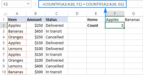
This technique works fine for a couple of criteria, but adding three or more COUNTIF functions together would make the formula too cumbersome. In this case, you'd better stick with one of the following alternatives.
Formula 2. COUNTIF with array constant
Here's a more compact version of the SUMIF with OR conditions formula in Excel:
The formula is constructed in this way:
First, you package all the conditions in an array constant - individual items separated by commas and the array enclosed in curly braces like {"apples", "bananas', "lemons"}.
Then, you include the array constant in the criteria argument of a normal COUNTIF formula: COUNTIF(A2:A10, {"apples","bananas","lemons"})
Finally, warp the COUNTIF formula in the SUM function. It is necessary because COUNTIF will return 3 individual counts for "apples", "bananas" and "lemons", and you need to add those counts together.
Our complete formula goes as follows:
=SUM(COUNTIF(A2:A10,{"apples","bananas","lemons"}))

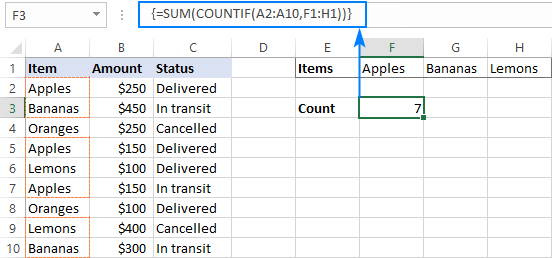
If you'd rather supply your criteria as range references, you'll need to enter the formula with Ctrl + Shift + Enter to make it an array formula. For example:
=SUM(COUNTIF(A2:A10,F1:H1))
Please notice the curly braces in the screenshot below - it is the most evident indication of an array formula in Excel:
Formula 3. SUMPRODUCT
Another way to count cells with OR logic in Excel is to use the SUMPRODUCT function in this way:
To better visualize the logic, this could also be written as:
The formula tests each cell in the range against each criterion and returns TRUE if the criterion is met, FALSE otherwise. As an intermediate result, you get a few arrays of TRUE and FALSE values (the number of arrays equals the number of your criteria). Then, the array elements in the same position are added together, i.e. the first elements in all the arrays, the second elements, and so on. The addition operation converts the logical values to numbers, so you end up with one array of 1's (one of the criteria matches) and 0's (none of the criteria matches). Because all the criteria are tested against the same cells, there is no way any other number could appear in the resulting array - only one initial array can have TRUE in a specific position, others will have FALSE. Finally, SUMPRODUCT adds up the elements of the resulting array, and you get the desired count.
The first formula works in a similar manner, with the difference that it returns one 2-dimentional array of TRUE and FALSE values, which you multiply by 1 to convert the logical values to 1 and 0, respectively.
Applied to our sample data set, the formulas take the following shape:
=SUMPRODUCT(1*(A2:A10={"apples","bananas","lemons"}))
Or
=SUMPRODUCT((A2:A10="apples") + (A2:A10="bananas") + (A2:A10="lemons"))
Replace the hardcoded array constant with a range reference, and you will get even a more elegant solution:
=SUMPRODUCT(1*( A2:A10=F1:H1))

Note. The SUMPRODUCT function is slower than COUNTIF, which is why this formula is best to be used on relatively small data sets.
Count cells with OR as well as AND logic
When working with large data sets that have multi-level and cross-level relations between elements, chances are that you will need to count cells with OR and AND conditions at a time.
As an example, let's get a count of "apples", "bananas" and "lemons" that are "delivered". How do we do that? For starters, let's translate our conditions into Excel's language:
- Column A: "apples" or "bananas" or "lemons"
- Column C: "delivered"
Looking from another angle, we need to count rows with "apples and delivered" OR "bananas and delivered" OR "lemons and delivered". Put this way, the task boils down to counting cells with 3 OR conditions - exactly what we did in the previous section! The only difference is that you'll utilize COUNTIFS instead of COUNTIF to evaluate the AND criterion within each OR condition.
Formula 1. COUNTIFS + COUNTIFS
It is the longest formula, which is the easiest to write :)
=COUNTIFS(A2:A10, "apples", C2:C10, "delivered") + COUNTIFS(A2:A10, "bananas", C2:C10, "delivered")) + COUNTIFS(A2:A10, "lemons", C2:C10, "delivered"))
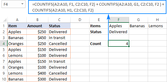
The screenshot below shows the same formula with cells references:
=COUNTIFS(A2:A10, K1, C2:C10, K2) + COUNTIFS(A2:A10, L1, C2:C10, K2) + COUNTIFS(A2:A10, M1,C2:C10, K2)
Formula 2. COUNTIFS with array constant
A more compact COUNTIFS formula with AND/OR logic can be created by packaging OR criteria in an array constant:
=SUM(COUNTIFS(A2:A10, {"apples","bananas","lemons"}, C2:C10, "delivered"))
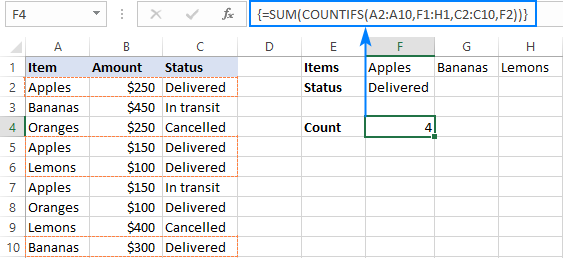
When using a range reference for the criteria, you need an array formula, completed by pressing Ctrl + Shift + Enter:
=SUM(COUNTIFS(A2:A10,F1:H1,C2:C10,F2))
Tip. If needed, you are free to use wildcards in the criteria of any formulas discussed above. For example, to count all sorts of bananas such as "green bananas" or "goldfinger bananas" you can use this formula:
=SUM(COUNTIFS(A2:A10, {"apples","*bananas*","lemons"}, C2:C10, "delivered"))
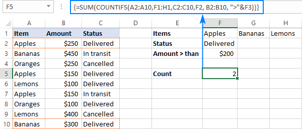
In a similar manner, you can build a formula to count cells based on other criteria types. For example, to get a count of "apples" or "bananas" or "lemons" that are "delivered" and the amount is greater than 200, add one more criteria range/criteria pair to COUNTIFS:
=SUM(COUNTIFS(A2:A10, {"apples","*bananas*","lemons"}, C2:C10, "delivered", B2:B10, ">200"))
Or, use this array formula (entered via Ctrl + Shift + Enter):
=SUM(COUNTIFS(A2:A10,F1:H1,C2:C10,F2, B2:B10, ">"&F3))
Count cells with multiple OR conditions
In the previous example, you have learned how to test one set of OR conditions. But what if you have two or more sets and you are looking to get a total of all possible OR relations?
Depending on how many conditions you need to handle, you can use either COUNTIFS with an array constant or SUMPRODUCT with ISNUMBER MATCH. The former is relatively easy to build, but it is limited to only 2 sets of OR conditions. The latter can evaluate any number of conditions (a reasonable number, of course, given Excel's limit to 255 arguments and 8192 characters to the total formula length), but it may take some effort to grasp the formula's logic.
Count cells with 2 sets of OR conditions
When dealing with only two sets of OR criteria, just add one more array constant to the COUNTIFS formula discussed above.
For the formula to work, one minute but critical change is needed: use a horizontal array (elements separated by commas) for one criteria set and vertical array (elements separated by semicolons) for the other. This tells Excel to "pair" or "cross-calculate" the elements in the two arrays, and return a two-dimensional array of the results.
As an example, let's count "apples", "bananas" or "lemons" that are either "delivered" or "in transit":
=SUM(COUNTIFS(A2:A10, {"apples", "bananas", "lemons"}, B2:B10, {"delivered"; "in transit"}))
Please note the semicolon in the second array constant:

Because Excel is a 2-dimentional program, it is not possible to construct a 3-dimentional or 4-dimentuional array, and therefore this formula only works for two sets of OR criteria. To count with more criteria, you will have to switch to a more complex SUMPRODUCT formula explained in the next example.
Count cells with multiple sets of OR conditions
To count cells with more than two sets of OR criteria, use the SUMPRODUCT function together with ISNUMBER MATCH.
For example, let's get a count of "apples", "bananas" or "lemons" that are either "delivered" or "in transit" and are packaged in either "bag" or "tray":
=SUMPRODUCT(ISNUMBER(MATCH(A2:A10,{"apples","bananas","lemons"},0))*

ISNUMBER(MATCH(B2:B10,{"bag","tray"},0))*

ISNUMBER(MATCH(C2:C10,{"delivered","in transit"},0)))
In the heart of the formula, the MATCH function checks the criteria by comparing each cell in the specified range with the corresponding array constant. If the match is found, it returns a relative position of the value if the array, N/A otherwise. ISNUMBER converts these values to TRUE and FALSE, which equate to 1 and 0, respectively. SUMPRODUCT takes it from there, and multiplies the arrays' elements. Because multiplying by zero gives zero, only the cells that have 1 in all the arrays survive and get summed.
Th screenshot below shows the result:

This is how you use the COUNTIF and COUNTIFS functions in Excel to count cells with multiple AND as well as OR conditions. To have a closer look at the formulas discussed in this tutorial, you are welcome to download our sample workbook below. I thank you for reading and hope to see you on our blog next week!
Practice workbook
Excel COUNTIF with OR conditions - examples (.xlsx file)
 by
by
121 comments
Hi there,
This is a great tutorial. I have something that I need a solution for.
I have 3 columns, Process (column A), Work Started (Column B), and Work Completed (Column C).
I need to know how many "Environmental Screening" Processes in Column A were worked on and/or completed in "2024/1st". I need it to count an environmental screening as 1 if it has "2024/1st" in column B OR column C, but also count an environmental screening as 1 if it has "2024/1st" in column B AND column C, I don't want to count a single environmental screening twice. I hope that makes sense.
I was thinking that I needed to string together an AND function and OR functions to accomplish this; an OR function for the (Work Started = "2024/1st") + (Work Completed = "2024/1st") nested into an AND function along with (Process = "Environmental Screening"). However, I can't seem to create a formula without getting an error message.
Any insight is appreciated
Hello Joe!
In your case, to calculate values based on conditions, use SUMPRODUCT function.
=SUMPRODUCT((A2:A100="Environmental Screening") * ((B2:B100="2024/1st")+(C2:C100="2024/1st")>=1))
or
=SUMPRODUCT((A2:A100="Environmental Screening") * ((B2:B100="2024/1st") + (C2:C100="2024/1st") > 0))
You can find more examples and detailed instructions here: Excel SUMPRODUCT function with multiple criteria.
Hi – I generate a list of stock symbols in an array (D20#) from the following formula:
=FILTER(Journal[Symbol],(Journal[$ P&L]>0)*(Journal[Entry
Date]>=$C$3)*(Journal[Entry
Date]0)*(Journal[Entry
Date]>=$C$3)*(Journal[Entry
Date]<=$E$3)))
Subsequently I use a formula =COUNTIF(D20#,C20#) to count the number of times a particular stock is present. However, I am unable to develop a single cell formula to make the calculation in Step 3 (Countif). Can you please guide me? Thanks.
Hi! In Excel formula =COUNTIF(D20#,C20#) uses spilled range references (#), meaning that D20# and C20# represent dynamic arrays.
However, COUNTIF does not support array references directly. Instead, you can use SUM formula with a logical condition:
=SUM(--(D20#=C20#))
This formula compares values in both arrays and counts the matches.
If you need to count occurrences based on a specific condition, SUMPRODUCT function can be useful:
=SUMPRODUCT(--(D20#="condition"))
Hi Alexander, this is the BEST tutorial! But I must be doing something wrong, because I cannot get this to work for me. Of course, I am trying to do something more complicated!
I want the formula to read a text in Column I, and return "Week 2", "Week 3" etc in another column for easy filtering. I was thinking/hoping that this would work: =COUNTIFS(I2,"Week 2"&"*"),"Week 2",(I2,"Week 3"&"*"),"Week 3",(I2,"Week 4"&"*"),"Week 4",(I2,"Week 5"&"*"),"Week 5",(I2,"Week 6"&"*"),"Week 6",""))))
But it doesn't, and I cannot get Excel to even accept the formula (I get a "There's a problem with this formula" message which doesn't help me in the slightest). Once I get this working, I will drag this formula down the 3000 lines of data.
Is there something obvious that I have done incorrectly?
Hello Sam!
Use the nested IF formula and these instructions: Excel IF statement for partial text match (wildcard). For example:
=IF(COUNTIFS(I2,"*"&"Week 2"&"*"),"Week 2", IF(COUNTIFS(I2,"*"&"Week 3"&"*"),"Week 3",""))
I would like to no if there is a formula that I can use, to identify where a date exceeds another date (all dates are different) and where true to count only for a specific person and exclude where another date is given. The due date remains the same but is different from each row of data. To try to be clear
A1:A50 - contains the due date
B1:B50 - contains the submission date
C1:C50 - contains the person the task is allocated to
D1:D50 - contains where a new date has been given and would need to exclude this from the total.
So I want to count when the submission date exceeds due date and only count if it is a certain person and not count if there is another date given.
In my mind, it should be easy but there is clearly something that I am missing as I only come up with 0 (which is incorrect) or an invalid formula. Please help
Hi! Here is a formula that counts the number of times the submission date exceeds the due date for a specific person, excluding rows where another date is given:
=SUMPRODUCT((B1:B50>A1:A50)*(C1:C50="Specific Person")*(D1:D50=""))
(B1:B50>A1:A50) checks if the submission date exceeds the due date.
(C1:C50="Specific Person") checks if the task is allocated to a specific person.
(D1:D50="") checks if cell is empty.
SUMPRODUCT function multiplies these conditions together and sums the results, effectively counting the rows where all conditions are met.
EX 1,2,3 this following text , we need to sepatate
1,2,3
2,1,3
3,1,2
3,2,1
2,3,1
1,3,2 - This formet - How to I do this
Hi! The answer to your question can be found in these articles: How to split cells in Excel: Text to Columns, Flash Fill and formulas and Split string by delimiter or pattern, separate text and numbers.
You can also separate text by cell using a single TEXTSPLIT formula:
=TEXTSPLIT(A1,",")
You can solve the problem without using formulas. Pay attention to the Split Text tool. If text is separated by commas, spaces, dashes, or other characters, you can use this tool to create multiple columns or rows from a single cell. It is available as a part of our Ultimate Suite for Excel that you can install in a trial mode and check how it works for free.
Hello Alexander,
Thank you so much for your GREAT tutorial.
This really really help my work life more easier, especially for "COUNTIF with array constant"
The formulation is workable for several wording criteria. But it's not workable when I combined different type of criteria, which is date & wording.
Such as, this criteria ">"&TODAY(). I would like to count items which included status "date after today" or "TBC".
Could you please help to sharing solution for make this workable "=SUM(COUNTIFS($I:$I,{">"&TODAY(),"TBC"}))?
Thank you in advance for your great suggestion :)
Hi! If I understand your task correctly, the following formula should work for you:
=COUNTIFS($I:$I,">"&TODAY())+COUNTIFS($I:$I,"TBC")
Here is the article that may be helpful to you: How to use Excel COUNTIFS and COUNTIF with multiple criteria.
A couple questions:
1. When applying multiple 'OR' criteria to a range, can one supply both text and cell reference criteria in a compact format, i.e., something like:
=SUM(COUNTIF(A2:A10,{$F$1,"bananas","lemons"}))
=SUM(COUNTIF(A2:A10,{&$F$1,"bananas","lemons"}))
My Excel 2010 doesn't like these formulas. Is there another way using countif to apply multiply OR criteria to a range without adding multiple countifs together using +?
2. Does Excel allow one to use functions within criteria in countif? Specifically, I would like to use not(), isblank(), left(), etc. I am thinking something like:
=SUM(COUNTIF(A2:A10,not($F$1)))
=SUM(COUNTIF(A2:A10,left($F$1,6)))
Thanks.
Hello! To apply multiple 'OR' criteria to a range, you can use the SUMPRODUCT function. For example:
=SUMPRODUCT(--(A1:A10={"bananas","lemons"}))
Look for the example formulas here: Excel SUMPRODUCT function with multiple criteria.
You can use separate operators and functions within the COUNTIF criterion. Learn more here: COUNTIF function in Excel - count if not blank, greater than, duplicate or unique.
You can perform similar calculations using the SUMPRODUCT function:
=SUMPRODUCT(--(A1:A10<>"bananas"))
You can also count partial matches with the criterion:
=SUMPRODUCT(--ISNUMBER(SEARCH(LEFT(F1,6),A1:A10)))
For more information, please read: How to find substring in Excel
I am trying to get my excel sheet to read ab=30 minutes and for the row to be read and automatically apply if there are 4 abs in the entire row, that it would show total time of 120 minutes. If that makes sense.
Hi! Sorry, I have no idea exactly what the task is. Please describe your problem in more detail. Write an example of the source data and the result you want to get.
I am trying to check three columns (say, A, B and C) for a particular region and, if the region it appears in any of the columns, then it should check a fourth column (say D) for another criteria (outcome) and count how many rows meet the outcome criteria. That would be simple if a particular region only appeared in column A or B or C. The problem I have is that the region may appear in one row in both columns A and B but I don't want it to count that as two (i.e. it must only count the region once if it appears in any of the three region columns AND meets the outcome). But if it appears in only column B and meets the outcome criteria, then it also only counts once. I've tried many ways to do this and just cannot seem to get it to work but I know it must be do-able.
Hi! If my understanding is correct, the following formula should work for you:
=SUMPRODUCT(((A1:A10=F1)+(B1:B10=F1)+(C1:C10=F1)>0)*(D1:D10=F2))
The following tutorial should help: Conditionally count / sum / average cells with multiple criteria.
Thank you SO much! That worked!
I need formula for differentiating duplicate values in column with integer in the end. For example, if there are 3 duplicate values in column i.e. "Apple" and I want to differentiate word "Apple" with "Apple-1", "Apple-2", "Apple-3" in next column.
Hi! If I understand your task correctly, try to use the recommendations described in this article: How to count duplicates in Excel. Based on your information, the formula might look something like this:
=A1&"-"&COUNTIF($A$1:A1,A1)
Thanks, query solved.
I have a spread sheet with two columns that I want to COUNTIF with if an OR statement is true.
The two columns (Call them A and B) both have optional values of "Y", "N", or blank. I want to set up a count of the number of rows where either column's value is "Y". Also I would like to display that as a percentage of 'Not Blank' (i.e. anything in column A or B)
For Example if A1,2 and 3 are "Y", B3 & 4 are "Y", B5 is "N" and A&B 6 are blank then the count returns "4" and the percentage "80%"
Hi! To count values by condition, use the COUNTIF function. Try to use the recommendations described in this article: COUNTIF function in Excel - count if not blank, greater than, duplicate or unique. For example:
=COUNTIF(A1:B5,"Y")
=COUNTIF(A1:B5,"<>")
From these values, you can calculate the percentage you need using these guidelines: How to calculate percentage in Excel.
I have a monthly spreadsheet with classes from various teachers, in three periods of the day and in various classes. I'm trying to use conditional formatting to color the teacher's name red, in case I mistakenly put that teacher in different classes but on the same day and at the same time of day. I can do it for one day, but I would like to know if there would be a way to do it for days 1 to 31 in a single rule, or would I have to do each rule for one day?
I'm using the rule:
=COUNTIFS($B$2:$B$11;$B2;$C$2:$C$11;$C2)>1
Ex:
classes days 1 2 3 ...
class 1 morning John Mary Peter ...
class 2 afternoon Peter Mary Peter ...
class 3 night Mary John Paul ...
class 4 morning Mary Peter Mary ...
class 5 afternoon John Mary John ...
class 6 night Paul Mary Mary ...
class 7 morning Peter John John ...
class 8 afternoon Mary John Paul ...
class 9 night John Paul Peter ...
class 10 morning John Paul Peter ...
Hi! Copy the conditional formatting to other columns using these instructions: How to copy Excel conditional formatting.
classes days -> 1 2 ... 31
class1 morning John Mary Peter ...
class2 afternoon Peter Mary Peter ...
class3 night Mary John Paul ...
class4 morning Mary Peter Mary ...
class5 afternoon John Mary John ...
class6 night Paul Mary Mary ...
class7 morning Peter John John ...
class8 afternoon Mary John Paul ...
class9 night John Paul Peter ...
class10 morning John Paul Peter ...
Hi if I have an array that could contain three different YouTube versions in any of the cells, and I want to count how many cells contain ANY version of YouTube (there are 3 different versions), my COUNTIF function isn't working accurately. It's telling me that 65 cells have it, but on hand/manual count I know I have only 61 cells that have it. The issue is, some cells have multiple versions of YouTube in the same cell, and it's aggregating them all instead of just counting that cell ONCE. Any idea how fix? Please and thank you.
I think I understand your problem, as my problem was similar. After a lot of searching around, I've devised a workaround that is this:
Add a column in your dataset that is set to either 0 or 1 based on whether any of the three different versions of youtube exist. Do this with an IF statement with an OR in the logical test part of the IF statement.
Then base your COUNTIF criteria on that column, not the column containing the YouTube information itself.
I hope that makes sense and is helpful.
Hello, I am creating a tracker to account for number of tickets purchased based by pay grade in this example E8 is the paygrade. I am also trying to account for number of tickets purchased by that paygrade as their guest and I am completely lost. I don't know what to put in the ??????? spot or if this is even the correct formula.
Example, John's paygrade is E8 who purchased 1 ticket for himself and 2 guest tickets, Michael's paygrade if E8 who purchased 1 ticket for himself and 3 guest tickets. I want to produce one cell that will count total number of E8's who purchased a ticket and the cell next to it I want to count total number of guest tickets purchased by all E8's. So one cell should have (2) and the cell adjacent should have (5) for this example.
Hi! Unfortunately, this information is not enough to recommend a formula to you. To count the number of values that match the condition, use the COUNTIF function. Look for the example formulas here: COUNTIF function in Excel - count if not blank, greater than, duplicate or unique.
if columns B1,2,4 are Y and B,3 is N, what formula will give me a % of meetings attended for a 12 month period
Hi! To count the number of "Y" in column B, use the COUNTIF formula.
=COUNTIF(B1:B100,"Y")
To find the number of all values, use the COUNTA function.
=COUNTA(B1:B100)
If you have forgotten how the percentage is calculated, use these instructions: How to calculate percentage in Excel.
I have a spreadsheet for degree summaries. For courses with prereqs I want it the add the prereq courses only if students have an A, B, or C. A couple courses have four prereqs. Currently, it's counting if a prereq is not blank, and then I have to double-check the grade, which can lead to errors. Is this possible?
You can specify the prereqs with "countifs" rather than "count". countifs, counts values with a condition to it. So for example, if you need a person with greater than 80 grades, in countif you select the range first then give it a condition separated by a comma.
I have a spreadsheet where I am using the following countifs formulas: =COUNTIFS(LOG!$H$2:$H$1249,"*Initial*",LOG!$K$2:$K$1249,"Anderson*")
I also need to add in one more item to consider: how may of those were received in a certain month. How would I do that?
Hi! I don't know how your dates are written down, but this instruction may be helpful: COUNTIFS and COUNTIF with multiple criteria for dates
Hi ,
Let's say I have 2 columns Column A - 1-20 and Column B - 31 - 50. How can I count the unique entries when column A is > 10 or Column B is > 40. Kindly help.
Hello!
If I understand your task correctly, the following tutorial should help: Count unique values with criteria.
Hi
My current issue is i have to sheets lets say
Sheet1 is where the formula is so
Countif(sheet2A:A;$C$3) this formula will be in cell C5 and the C6,C7, C8
What i need is to move the auto fill series to move ranges on sheet2 to be filled as the formula on C6 to query B:B, C7 to query C:C and so on
Can you help me with that please
Hi!
Copying the formula down may change the row numbers, but not the column numbers. Autofill is not working the way you want.
You can dynamically change cell addresses in formulas using the INDIRECT function.
Hi, I'm trying to assemble multiple AND/OR logic. The first group I can solve with SUM(COUNTIFS, but getting stuck after the OR logic
Count cells if:
column F is one of: "*Scope*","*Component*","*Vendor*" AND column E = A2 (let's call this group1)
OR
column F = "*Decommission*" AND column I "*Production*" AND column E = A2 (let's call this group2)
Final result should be total cell count of group1 + group2
(wildcards intentional)
Thank you
note in the second group column I doesn't equal "*Production*" - looks like my symbols were removed