The tutorial explains what may cause a #SPILL error in an INDEX MATCH, VLOOKUP, SUMIF and COUNTIF formula and how you can efficiently resolve it.
It is sad enough when a brand-new feature refuses to work in your Excel. But even more frustrating is when a good old thing stops working all of a sudden, and you are receiving an error for a formula that worked perfectly for years.
The below examples show how to fix a few common formulas that got broken because implicit intersection is no longer invisibly performed in Excel. If you have never heard this term before, I encourage you to carefully read the #SPILL error tutorial to understand what is happening behind the scenes.
#SPILL error with Excel VLOOKUP formula
Here is a standard VLOOKUP formula that works fine in pre-dynamic Excel (2019 and earlier), and triggers in a #SPILL error in Excel 365:
=VLOOKUP(A:A, D:E, 2, FALSE)
As we can reasonably assume, the problem is in the first argument (the red reference above) that forces the VLOOKUP function to look up all the values in column A, which is over a million cells (the exact number is 1,048,576)! In the past, that was not a problem - Excel could only look up one value at a time, so it discarded all but one value in the same row as the formula. This behavior is called implied or implicit intersection.
With the introduction of dynamic arrays, all Excel functions got the ability to process and output multiple values, even those that were not initially designed to work with arrays! So, each time VLOOKUP receives an array of lookup values, it tries to handle them all. In case there isn't enough space to output all the results, you see a #SPILL error.
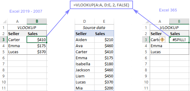
To resolve an Excel VLOOKUP spill error, you can use one of the following methods.
Look up range rather than column
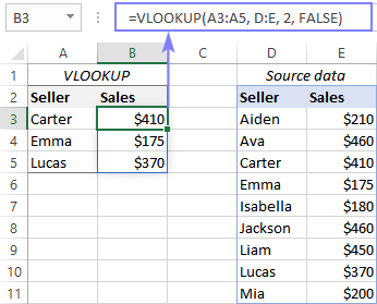
As we only have 3 lookup values, we limit the lookup_value argument to three cells:
=VLOOKUP(A3:A5, D:E, 2, FALSE)
The formula needs to be entered just in one cell and it will fill as many cells as needed automatically. The result is a spill range like this one:
Notes:
- If you are getting a #SPILL error anyway, make sure the spill range is empty, so nothing gets in the way.
- This solution does not work within an Excel table because tables do not support dynamic arrays.
Look up a single value
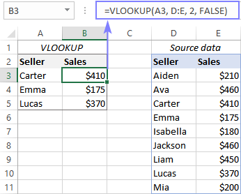
Write a formula for the first lookup value and copy it down through as many cells as needed:
=VLOOKUP(A3, D:E, 2, FALSE)
It is my preferred option as it is simplest to implement and works flawlessly in all Excel versions, from within normal ranges and tables.
Enforce implicit intersection
To limit an array to one lookup value, place the intersection operator @ before the column reference:
=VLOOKUP(@A:A, D:E, 2, FALSE)
As with the previous example, you enter the formula in one cell and drag it down the column.

Whichever solution you choose, a #SPILL error should be gone and your VLOOKUP formula starts working normally in Excel 365.
#SPILL error with Excel INDEX MATCH formula
In case you are using the combination of INDEX and MATCH functions to pull matches, a #SPILL error can arise for the same reason - there is insufficient white space for the spilled array.
For example, here's the formula that flawlessly returns sales numbers in Excel 2019 and earlier versions, but refuses to work in Excel 365:
=INDEX(E:E, MATCH(A:A, D:E, 0))
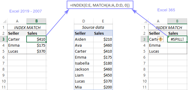
The remedy is already known - reduce the number of lookup values by applying one of the following techniques.
- Look up a range, not a column:
=INDEX(E:E, MATCH(A3:A5, D:D, 0)) - Look up a single value:
=INDEX(E:E, MATCH(A3, D:D, 0)) - Enable implicit intersection - add the @ character before a column reference, so that Excel processes only one value:
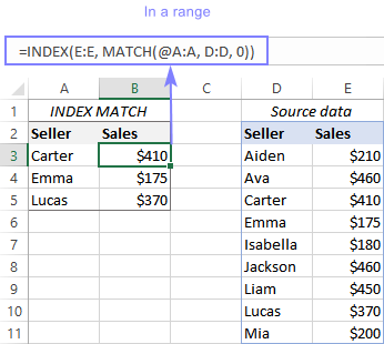
=INDEX(E:E, MATCH(@A:A, D:D, 0))
The result of the 1st formula is a dynamic spilled array, which is a great thing that saves you the trouble of copying the formula to other cells. The limitation is that dynamic arrays only work in a range, not a table.
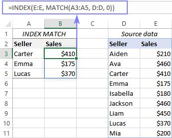
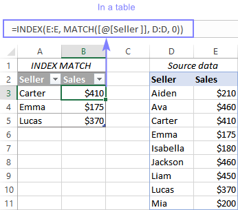
The 2nd and 3rd formulas return a single value, which a table can also accept. If your data is organized as a regular range, drag the formula down to copy it to the below cells. In a table, the formula will propagate automatically. In the latter case, you can also use a structured reference notation referring to the column headers:
=INDEX(E:E, MATCH([@[Seller ]], D:D, 0))
The below screenshots demonstrate the 3rd formula in action:
#SPILL error with Excel SUMIF and COUNTIF formula
When a SUMIF, COUNTIF, SUMIFS or COUNTIFS formula returns a #SPILL error, it might be caused by many different factors. The most often ones are discussed below.
Spill range is too big
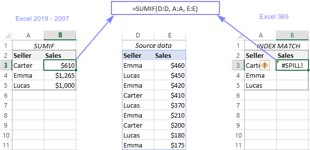
A very typical cause is supplying a whole column for criteria. Yep, that used to work in older Excel versions, but not anymore, since the new spilling feature produces nearly 1.05 million results and there is not enough space to accommodate them all!
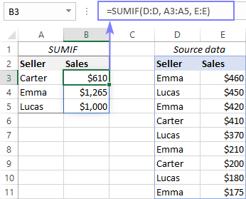
For this example, let's try to find a total of sales made by three vendors (A3:A5). In Excel 2019 and lower versions, you could successfully use the below syntax. In Excel 365, you will be getting a #SPILL error:
=SUMIF(D:D, A:A, E:E)
If you followed the previous examples closely, you know that the error can be resolved in three different ways:
- Use a range for your criteria, not a whole column:
=SUMIF(D:D, A3:A5, E:E) - Define a single cell for the criteria and copy the formula down:
=SUMIF(D:D, A3, E:E) - Include the implicit intersection operator (@) to limit the column reference to one cell:
=SUMIF(D:D, @A:A, E:E)In a similar fashion, you can get a count of sales for each person by using the COUNTIF function:
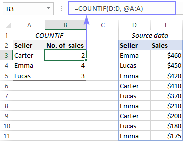
=COUNTIF(D:D, A3:A5)=COUNTIF (D:D, A3)=COUNTIF (D:D, @A:A)
Please remember that the 1st formula spills automatically into the below rows and can only be used within a range, not a table.
The 2nd and 3rd formulas return a single value, so you enter them in the first cell and then copy down the column as usual.
Criteria expressed incorrectly
The SUMIF and COUNTIF criteria are also a common source of problems. Sometimes, people overthink it and write the criteria as D3="carter" or D3:D11="carter" or D:D="carter". All three expressions are wrong and cause a formula to produce zero or a #SPILL error!
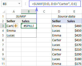
The correct way is either a range/cell reference like in the above examples, or text enclosed in quotation marks:
=SUMIF(D:D, "carter", E:E)
To learn more about what is acceptable in criteria and what is not, the following guidelines might be helpful: SUMIF criteria syntax.
Wrong order of arguments
In singular and plural versions of the SUMIF function, the order of arguments is different:
- With SUMIF, you first define range, then criteria, then sum_range (optional).
- In case of SUMIFS, the first argument should be the sum_range, and then range/criteria pairs.
If you muddle things up, a #SPILL error occurs.
In our example, criteria_range is D:D and sum_range is E:E. If you put one in place of the other, the formula will throw a #SPILL error again:
=SUMIFS(D:D, A3:A5, E:E)
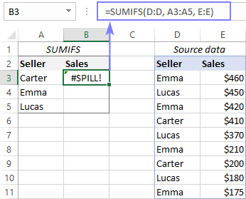
Arrange the arguments in the correct order, and SUMIF will give you the desired result:
=SUMIFS(E:E, D:D, A3:A5)
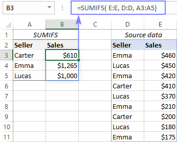
That's how to resolve a #SPILL error with Excel INDEX MATCH, VLOOKUP, SUMIF and other functions. I thank you for reading and hope to see you on our blog next week!
 by
by
7 comments
Hello,
I will agree this post is not related to #SPILL error but I urgently need help on this. Below is a representation of a formula I am computing using excel for this
f=1- (T_(ra(1))-T_ra(2) -…………..-T_(ra(n))) / (T_(loc(1))-T_loc(2) -……….-T_(loc(n)) )
=1-((F1860-O1860-X1860-AG1860-AP1860-AY1860-BH1860-BQ1860-BZ1860-CI1860-CR1860-DA1860-DJ1860-DS1860-EB1860-EK1860-ET1860)+(273.15*17)/('[Conversion.xlsx]CRIG TAFO'!AI1860-[Conversion.xlsx]KNUSTJHS!AI1860-'[Conversion.xlsx]OBUASI TSHS'!AI1860-'[Conversion.xlsx]Mountain High'!AI1860-[Conversion.xlsx]Dompoase!AI1860-[Conversion.xlsx]Bowdwensango!AI1860-[Conversion.xlsx]OFOASE!AI1860-[Conversion.xlsx]Bompata!AI1860-[Conversion.xlsx]Konongo!AI1860-'[Conversion.xlsx]St Monica'!AI1860-[Conversion.xlsx]Mankranso!AI1860-'[Conversion.xlsx]Kumasi Airport'!AI1860-'[Conversion.xlsx]Boa Amponsem'!AI1860-[Conversion.xlsx]Abono!AI1860-'[Conversion.xlsx]Kumasi SHS'!AI1860-'[Conversion.xlsx]KNUST FARM'!AI1860-'[Conversion.xlsx]IITA Mabang'!A-1860))
the issue here is that I have crossed checked the input and formula over and over again and there is nothing wrong but i keep getting #NUM! error. Please how do i solve it
Hello!
Unfortunately, without seeing your data it is difficult to give you any advice. It is very difficult to understand a formula that contains unique references to your workbook worksheets. Hence, I cannot check its work, sorry.
What are the possible things that may account for a #NUM! error. If you reference a lot of workbooks and sheets, are you bound to encounter errors?
What formula or command can be used, to count different items in a column from one sheet to row in another sheet, e. g counting all A's, B's, C's etc in Maths, Eng, Chem, in a column and move it to row in another sheet: e.g Maths 1A, 2B's 5C"s
Eng 2A"s, 3B"s, 7C's
Chem 4A's 5B"s 6C"s
kindly check; vlookup problem; for some reasons, sum will not go through; its a data sheet
A B C D E
1 0;13 0;00 required; zero
2 0;15 0;33 required; d2-sum(c1+c2)
3 0;32 0;41 required; d3-c3
4 0;16 0;00 required; zero
5 0;14 0;00 required; zero
6 0;20 0;00 required; zero
7 0;01 0;59 required; d9-sum(c4:c7)
8 0;14 0:00 required; zero
9 0;12 0;41 required; d9-c9
thanks
In Auto Fill in Excel the + sign at the bottom right of the cell does not appear
Hi!
Perhaps, the Auto Fill feature is turned off in your Excel. Here's how you can quickly turn it on: How to enable / disable AutoFill in Excel.