In this tutorial, you will lean a quick way to calculate percentages in Excel, find the basic percentage formula and a few more formulas for calculating percentage increase, percent of total and more. Continue reading
Comments on: How to calculate percentage in Excel - formula examples
 by Svetlana Cheusheva, updated on
Comments page 22. Total comments: 728
Dears
How to calculate % ?
23.06+6%-19%
Please help.
Br/Dhiraj
suppose Cell A1 contains units 1600...
in A2 write formula =A1*30%
in A3 formula =A1*40%
and so on..
I need help on a very simple formula
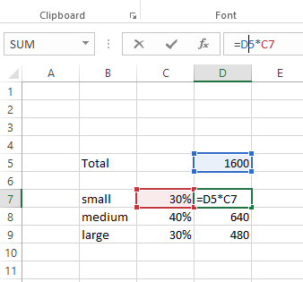
my customer orders x qty of an item. she orders in 3 sizes at a percentage.
ie. 1600 units
30% is size small
40% is size medium
30% is size large.
how can i set up a formula in excel where i can change the total units to figure this out? It is easy on a calculator, challenging in excel.
thank you!
dee
Hello, Dee,
Please have a look this picture:

Good morning. I need help. I want to create a formula that calculates percentages AFTER the first 6%. Currently I have it set up to calculate up to the first 6% but need to change it to only calculate everything AFTER the first 6%. =IF(B14>=0.06,"6%",IF(B14>=0.05,"5%",IF(B14>=0.04,"4%",IF(B14>=0.03,"3%",IF(B14>=0.02,"2%",IF(B14>=0.0001,"1%",IF(B14=0,"0%")))))))
Hello, Delane,
This formula should help:
=IF(AND(B14>=0.001,B14<0.02),1, FLOOR(B14*100,1)) & "%"
#DIV/0!
=(current month-previous month)/previous month this for increase and decrease formula
ok
now
=(3-0)/0 what is the answer pls. send ASAP
i have divided 16/0 and answer is #DIV/0!..can you please send me any formula to make this correct..
11/6/2015 11/7/2015 VARIANCE REDUCTION %
91 94 3 3%
19 28 9 47%
25 25 0 0%
20 5 -15 -75%
50 31 -19 -38%
11 9 -2 -18%
2 2 0 0%
1 1 0 0%
0 16 16 #DIV/0!
5 8 3 60%
4 4 0 0%
A B C D
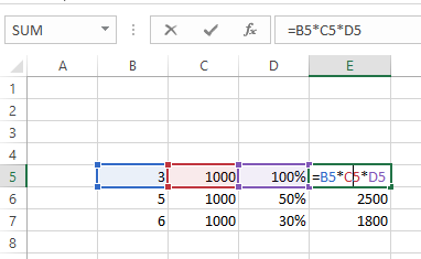
Unit Value Percentage Amount
3 1,000 100% 3,000
5 1,000 50% 2,500
6 1,000 30% 1,800
Can I know how to set the formula for Column D for the scenario above?
Hello, Jeanette,
Please see the formula you should use on the picture below:

I have to keep records of customer service dates.
How do I find the percentage of services completed.
I have a simple set. Months and the dates are in each cell corresponding to the customers name.
How at the end of the year do i calculate the amount of services completed?
I'm very confused.
i have a formula
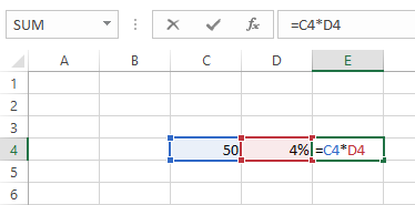
=C4*4%
I want to know if there is a way to add a formula without the number of percent and i can just add in 5% or 4% when ever i like i tried doing
=c4* ?%
but that doesnt work
Hello, Marisol,
Try this formula:

How can I have my average formula have to total to equal the original value eg.(I need to divide 626.27 by 80% 3& and 17% were the amount in the percent column are equal to $626.27) Some of my values are off by a penny, I assume that is a rounding issue, but I need to find a way around this.
Melissa
Hi.
How can Calculate automatic in tax value % as per detail.
For Exmaple:-Basic Value:-4000 on tax value :-400 Total value :-4400 total tax:-10%
But Every time i have manual type tax === 10% ,8 % ,15%, 5%. ( this is Example)
please help me that i want automatic show tax value there is automatic show tax % value.
Hi . I want to need some of formula how to paste for exam
Hi Svetlana,
Trying to help my husband do a spreadsheet for his work... I have a list of items and 3 regions with their separate totals for each item. The items are then totaled separately(all 3 regions together)to get the new total. There is a separate column to put the total out of 100% for each specific item. This column of totals then all need to add up to 100%. The only excel I have done is simple, not like this, so I'm lost - can you help me?
Thanks so much in advance.
Deb
Hello, Deb,
For us to be able to assist you better, please give us an exact example and describe the expected result. Thank you.
good morning
i need help with how to make a formula to calculate the percentage of total sales for different Quarters
Respected Madam,
Will you please how to find a formula in excel
My product rate : 255000
Net Discount Rate : 165000
percentage : ?
how to find how much discount less and percentage formula in excel
Product Price on cash basis less 10% Discount
if unit price is 1.65 i want to less 10% if i less this amount on excel sheet my remaining amount is 1.55% than i re-typed on my calculator i will received amount 1.48 tell me how do possible this accurate.
1. values In Excel, you have a list of values in cells A1 through A40. Explain in words or show the formula you would use to give the average of the.
helo i want to know how to calculate ms excel step by step
10 205 7 75.00%
13 205 7 75.00% a)what % of the sample
29 202 9 71.40% weigh 172 lbs or less
3 201 10 67.80%
11 200 11 64.20% b)what % of the sample
7 196 12 57.10% is 200 lbs or more
14 196 12 57.10%
25 195 14 50.00%
26 195 14 50.00%
19 193 16 46.40%
5 191 17 42.80%
12 174 18 39.20%
21 172 19 35.70%
24 165 20 32.10%
22 163 21 28.50%
9 162 22 25.00%
23 161 23 21.40%
18 159 24 17.80%
1 157 25 14.20%
6 156 26 7.10%
28 156 26 7.10%
16 152 28 3.50%
20 150 29 0.00%
in excel you have a list of values in cell A1 through A40 explain in words or show the formula you would use to give the average of the values.
pls gv me d ans
Good day every one.am a novice in excel. So pls I need your help on this question...you as a business manager is expected to manage and keep your clients records, client I'D, client name and amount credited are inputs from the user of the package while amount debited and balance are computed fields where amount debited is 10% of amount credited.use the the figure below and write the formulas for: Amount debited and balance when 10% of the amount credited is the amount debited and the balance is what remains after taking away the amount the amount debited from the amount credited...so pls I want to knw the formulas for amount debited and balance...... Thanks
HELLO EVERY ONE
Any one me teach me Excel classes
Hi
I need to make equation to convert percentage to points in excel Like that
- 60% to 70% = 2 points
- 71% to 100% = 3 points
- 101% to 120% = 4 points
- 121% to infinity = 5 points
thanks for your help
Hello Beshoy,
To display points corresponding to percentages, you can use a nested IF formula like this:
=IF(A1>120%,5, IF(A1>100%, 4, IF(A1>70%, 3, IF(A1>=60%, 2,""))))
- first thing thanks for your help
- second thing I need it but with Variable points not fixed
Exp : form 60% to 70% = 2 points Maximum If It equal 70%
If the percentage is 65 that means the points is equal part of the total points, but not all
Sorry, I an not sure I can follow you. The formula assigns 2 points for percentages between 60% to 70%, inclusive. Are you looking for something different?
Hi
I need to make equation to convert percentage to points in excel Like that
- From 60% to 70% = 2 points
If the percentage between 60% & 70% the point will be displayed according to the percentage Like that
1- IF the percentage less than 60% the point will equal 0 point
2- IF the percentage = 60% the point will be equal 1.0 point
3- IF the percentage = 65% the point will be equal 1.5 point, that means the is Variable not fixed
4-IF the percentage = 68% the point will be equal 1.8 point
Notes:
- total range for the percentage is 10%
- total point range is 2 Points
thanks for your help
Hi
Sorry I need your answer urgent
Hi everyone..
I have a query..How to calculate a series of percentage for whole excel in one go?? for eg. if column A(A1 TO A 30) deals with marks obtained by 30 students in exam and Column B shows the total marks. so is there a formula by which we can calculate the percentage of all students in one go and don't do (=A1/B1 setting percentage function)??
Hi Anoop,
Sorry, I am not sure I can follow you. If =A1/B1 is the right formula for calculating the percentage of total for each student, and all you have to do is copy that formula down to other cells in the column. If the total is in some particular cell in column B, say B1, add absolute sell references like =$A1/$BS1 for the formula to copy correctly.
Hello Shahid,
Here you go:
=100*6+(100*6)*0.01
I need an Excel formula for this - if i charge 3% for every $10 i loan for 2 weeks, how much will I earn for $200 I loan for 2 weeks
100×6+1%=606
How can i get this answer in excel.
Tell me formula to get this answer.
In Cell B14, calculate the Cost of Sales by multiplying the Sales Amount 60%. (Hint; In your formula, multiply the value in cell B6 times.6.) Copy the Formula to the range C14:E14.
I'm sorry I am trying to figure this out. Like i know that there is a hint there but at the same time this is my first time doing this. Can someone help me asap before the night is over I would appreciate it
Hello,
I have to keep track of all the annual training for all the employees. The employess that have finished a training I mark the cell green, and for the training not yet completed I mark the cell red. I want to calculate percentage of green cells. How do I do that?
Thank you very much!
Iza
You can use this formula for quick understand:-
For eg.,
Given amount is Rs. 18000. Interest 3%.
Answer = (18000/100*3), is 540.
Dear sir,
please post easy percentage formula
I have a total increase of 5%. Product A increased by 9%, Product B increased by 7%. How can I tell how much % Product A and B contributed to the overall increase?
i have 14% but i want it to show as -84% what formula do i put it to make it show this?
Hi Vicki,
You probably meant -14%? To reverse the sign, you can simply multiply the value by -1, e.g. =A1*-1
If you want to reverse the sign in existing cells, you can use the Paste Special function:
- Enter -1 into any blank cell, and then copy that cell.
- Select the range of cells where you want to change the sign.
- Right click the range, select Paste Special > Multiply.
sorry i meant i want it to say -86%
Hi,
if i have number 811 then how to calculate 5.20% out of them.
Regards,
Rajeev Mishra
Hi Rajeev,
This is the general formula:
Total * Percentage = Amount
In your case, =811*5.2% or =811*0.052
Either way, the result is 42.172.
i need a percentage of pass + fail. I have 10 tests, 3 pass and 4 fail. What is the % that was tested?
Hi Sammy,
You can use the following simple formula, replace values with corresponding cell references, and apply the percentage formal to the cell with the formula:
=(3+4)/10
Hi everyone,
I am building a spreadsheet with a number of columns holding information regarding audits that have been carried out on various establishments. About 10 of the columns will relate to regulatory articles and may or may not have a numerical figure entered in the row to the related establishment. What I want to do is find the percentage of rows within that column that have an entry against the total of audits (number of rows) completed.
Hope someone can be of help.
Many thanks.
Hi,
I want to calculate in percentage the adherence to plan in the work place
Example 1: Planned 100 CTNS VS actual 90 Ctns = 90%
Example 2: planned 100 Ctns VS Actaul 110 Ctns = because it was overproduced, i want the formula to calculate the inverse result, no 110%
Hi,
Hope you can help me on this, I have a spreadsheet with the left and right margins set at 0 and top and bottom set at 0.25. My paper size is 8 1/2x11” Landscape. My work is within the margins but when I do a print screen it shows 2 pages to print. The second page is blank. I am not sure way this happens.
Thanks
What a great article. As an example I would like to track percentage of sales Ytd vs lytd
Customer x spent 25,000 last year and I have put in a 10% budget increase and this ytd has spent 8,000 what formula would I use to calculate percentage of budget ytd
Thanks
Hi, I have a question, I am trying to calculate up a percentage and can't figure out the formula… can you help me?
I have a wholesale price of $25
I know the retailer wants to make 20%
How do I calculate the consumer price - but if I times 25x20%, i only get $5, and added to the original $25 is $30. But 20% of $30 is $60. I can't figure out the formula in Excel. Thanks!
Karin,
$5 is 20% of $25.00 total. 20% of $30.00 is $6 not $60.
(where A1 is the total of $25) you will enter the following in B1 =A1x5%
use the * not the x in the cell B1 ...sorry just noted that after it posted.
i wanna buy something..86500 that's the price..but the seller says that he will give me 50% + 20% off..what does it meant?? how much should i pay? n how to make the formula ??
i wanna buy something..62.23 that's the price.and tax price is 12% where as rate is 66.23 how to write a formula on excel ....
Most likely your price is 34600:
=86500*50%*(100%-20%)
or
=86500*0.5*0.8
But you'd better check with the seller anyway because the offer is not crystal clear...
that's the formula i need...thank you very much Ms.svetlana
i have multiple percentage 50% + 20% off from the price list..how to make the formula to know how much should i pay??..thanks before
Hi Ali,
If you want to calculate the discounted price, you can use a formula similar to this: =A1*(100%-20%)
Where A1 is the full price and 20% is the discount.
If you are looking for something different, please clarify.
i wanna buy something..86500 that's the price..but the seller says that he will give me 50% + 20% off..what does it meant?? how much should i pay? n how to make the formula ??
I have cells in multiple non-consecutive columns(all on the same row) that I need to total, others identical that I need to total and then find a percentage of the difference between those two totals. IE: Total merits/total demerits= what%.
The reason is because they are broken down into individual sections(columns) that already display a %, now I need an overall %. Hope that is enough info. Thanks!
I'm try to get an equation like this can you guys for my excel help ..
Example
1075*7% + 5% + 70+ 45 +108 =342 .
In other word
$1,075 * $75 +$54+70+45+108 =342
Hello, I need some help creating a % increase
Im looking to have column "F" increased by 12%, so that column "G" shows the product
I can not seem to get the formula correct.
Hi, I hope you are fine.
I have cities two month sales and percentage of two months sales. after I want to give 900 TV give form all cities by percentage of sales. when I drag it not show me correct.
TVGift 900
City Month1 Month2 Percentage
Kabul 100,000 490000 20% 184
Mazar 200,000 490000 41% 75
Badghis 120,000 490000 24% 18
Farah 30,000 490000 6% 1
Helmand 40,000 490000 8% 0
490,000 100% 278
In here must be 100% Not correct.
Best regards
Am very much happy to learn from excel sheet. I do hope to learn more its great helpful to me.
Kindly also send me thru my email on how to work more on calculating pls
With regards,
Henh
If I wanted to get percentage of Pass per month? For example In January with 31 days X person achieved the goal (passed) 18 days which would be 58% percent for January for that person. Any ideas would be appreciated. There are 23 employees being track on one spreadsheet, per day, with a pass or fail grade. I tried a pivot table but its not what I need. Thanks!!!
This is all very helpful. Thanks!
Column A of per person cost.
Column B of number of people.
I need to multiply the per person cost by the number of people. THEN add 8.25% sales tax to the multiplied amount.
Per Person x number of people + 8.25% sales tax.
I cannot figure it out for the life of me. Please help.
Hi Danny,
Here you go:
=A2*B2+(A2*B2)*8.25%