In this article, you will find two quick ways to change the background color of cells based on value in Excel 2016, 2013, and 2010. Also, you will learn how to use Excel formulas to change the color of blank cells or cells with formula errors. Continue reading
Comments on: Two ways to change background color in Excel based on cell value
 by Svetlana Cheusheva, updated on
Comments page 8. Total comments: 426
Thank you very much.
This Article is very helpful and it contains many solutions for excel.
Am prepare timeline chart for project. i need to highlight sundays dates.how to color Sundays by conditional format
I have 2 column's one for start date and the other end date - and next coloum gives the numbers of days between the start date and end date ..
if i say
Column E -- start date
Column F -- End Date
Column G -- no of days
If i want to get the cells in Coloumn G coloured for all the row which donot have a end date ..... how can I format it .
This is awesome, thank you.
I am wondering: I have a group of cells in which I have numbers, and I am usin the MIN command to find the lowest number between these cells. I would like to have a cell next to the one displaying the lowest number then display a block of text and a cell color based on which of these cells has the lowest number, so I can basically show a "winner" of which number is the lowest in the data set. Is this possible?
So essentially it looks like:
1 2 3
Thank you!
I would like to conditionally format cells that contains a date, based on values in different cells. My cell contains a date (indicates due date) and the gradient bar behind it would indicate percentage complete in color (stored in a different cell). Can you provide some help please?
I want line charts details ,with green colour line shows if its upward and red colour line shows if its Downward ,one line in one chart
I want chart details for I use two column plan and actual, plan > actual green colour ,and plan < red colour , how to form methed
Hi Svetlana,
Actually i am in "sheet1 cell a1" and I want this cell colour to be changed based on the value of "sheet3 cell n12". Can you please help me out. Thanks
Thanks I got just now...
This article is super helpful. I'm trying to do something based off of your writings and...it's not working. I wonder if I'm going about things completely wrong.
I have a list of student levels on a worksheet from one semester, I have made a duplicate for the next semester, the new values are entered in semester 2 - and want anybody who has moved up to level 4 (Levels run 0 Bad to 4 Achieved) to be highlighted green.
I.e. If you have moved up to level 4 between semesters, you are colored green.
I tried conditional format in the second semester
=AND(Semester1!$A$1:$D$29<4,Semester2!$A$1:$D$29=4)
Format: Fill Green
I don't know if it's because the data is on two sheets (I could put it on one) or if it's the way I'm using the range. Or that I'm being too basic and should just color in the cells myself!
Sorry if I have gotten all this completely wrong. It's nice to find someone on the interweb who makes sense!
Stephanie
Hello, Stephanie,
To help you better, we need a sample table with your data in Excel. You can email it to support@ablebits.com. Please add the link to this article and your comment number.
Thanks,
It is really useful for us ...
Thanks again
i want this cell number 1 to 100 but 15 is grater then color green and other red color then use formula excel sheet
DEAR SIR,
I AM USING ONE IF CONDITION FORMULA, WHICH RESULT IS PASS OR FAIL.
I NEED THE RESULT WITH COLOR. EXAMPLE.PASS WITH GREEN BACKGROUND AND FAIL WITH RED COLoUR
Thanks a lot for adding the drops of knowledge in my excel skills,
I respect as like as Teacher,
This help me. Thank you
Many Thanks Easy to understand.
I would like to highlight cells which end in a certain number. Cells ending w/ 0,1,2 colored yellow; 3,4,5 green and so on
Hello, Shawn,
Please see the picture below:
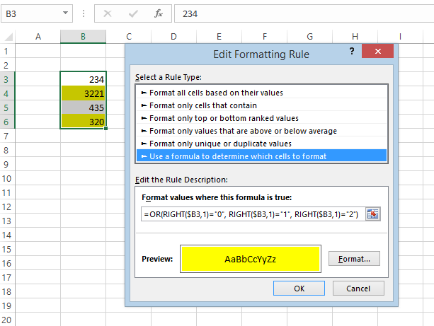
Hope this helps.
i want whan type BUY than cell become Green and whan type SELL than cell become Red pls help on that
Hi,
i have one set of numbers in one cell ex: 32 48 52 55 57 59, now i want to color only 32 in this array
please let me know how to do......
i want whem i write the world ( done ) the raw will be automatically green .... how can i do that
Useful Article.Thanks...
I have three cells. If Cell A1 is blank AND cell A2 is also blank then cell A3 should have value of 1.00 with light grey color and if cell A1 is not blank AND cell A2 is not blank then the cell value of A3 should be 1.00 in black colour. How can I do this in Excel?
i got it thank you soo much
But the thing I want is instead of values if i keep letter or characters for which i want to change the color of whole row or colum
Hi Svetlana
Thank you for sharing knowledge it is more useful and easy for me by following your steps.
Thanks alot
Its very usefully for me
In cell m145 I have formula =sum (a1:a5,b3:b7,c4:c9,etc...)
I can not figure out how to click on m145 and command it to change all the cells in the formula to turn a certain color.
Help please.
Hello Svetlana - Thank you so much for offering your time to all of us...
I want to change the background color of an entire row to the color associated with the results of the conditional formatting of a cell in the row.
Thanks!
Hello Neil,
Just select the entire rows before creating a rule, or you can edit an existing rule and make sure it applies to all the columns you want to highlight.
You can find full details with screenshots and examples here:
https://www.ablebits.com/office-addins-blog/excel-change-row-color-based-on-value/
Thanks very much for your helpful article.
I want to change a range of cells based on the values of each equivalent adjacent one. For example.
A1 0
A2 1
A3 1
I want to change A1 only if its equivalent adjacent is 0, same rule for A2 and A3, get it?
I want to apply this for a range of cells, because my spreadsheet is really huge and apply this conditional formatting for each cell is really painful.
Thanks!
Hello. I am not 100% whether it has already been answered, so I'm sorry if the question is being repeated.
I want to be able to change a cell (i.e. someone's name to a different colour) if they have responded to me. Basically if they have not response cell is blank, I want the font colour of the persons name to be Red, and if they have responded and the response cell has some data in it, I want their name to become Green. How would I do this?
I hope that's clear enough? If not I can provide a clearer question.
Thankyou! :)
Thnx 4 the HELP......
Hi All,
I need help in excell my question is if i change a color in one cell of sheet
automatically it should change in another cell of another sheet.
Example:I have 6 sheets with same information.
In "Sheet1 Jan sales" "Sheet2 FEBsales".If I change color "Yellow" For "Sheet1 Jan sales"in A6 cell "YEs" it should same refelect in "Sheet2 FEBsales" in A6 cell "Yes" as Yellow.
Please send me with temp let with clear explanation.
Waiting for solution for my question
regards,
Lakshmi
This is great. You have explained it so easily. Thanks
Hi,
I want the following thing
If B2 is equal to D2 then the cells become Green
If B2 is equal to C2 then the cells become Red
Can you please tell me
Hi Svetlana,
What I am trying to achieve is a reporting tool.
I want to have default values and when they change, then have the cell display as red.
So the scenario is A1 = Yes, B1 = No
When the user changes either one, I'd want it to change colour. Is this done through conditional formatting?
Hi Will,
I think you can create 2 rules with the following simple formulas:
For column A: =$A1<>"yes"
For column B: =$B1<>"no"
superb .....its work.
thanks.
thanks!!!
Can I format a single cell or set of cells to highlight if another single cell or set of cells has any value? In other words, I have 5 cells that will contain data. If cells further down change from blank to any value (could be numeric or alpha or combo) I want the 5 cells with data to then be highlighted. Is that possible??
Hi All,
The numbers "Age" column should be filled in with colors against the status mentioned against each of them.
How can we do this using conditional formatting.
Say for example cell containing "3" should be filled with Orange color.
Age Status
3 Orange
4 Green
10 Red
Hello Dinesh
Here is your solution step by step
let me assume cell A2=3, A3=4 and A4=10
1. Go to cell B2
2. Click on Conditional Formatting
3. Select Manage Rules
4. Click New Rule
5. Select Use a formula to determine which cells to format
6. In the box of "Format values where this formula is true:" type
=A2=3
7. Click on format select fill and select the color you want
8. Click ok again ok and again ok
9. Go to Cell B3 and repeat step 2 to step 5
10. In the box of "Format values where this formula is true:" type =A3=4
11. Repeat step 7 and step 8
12. Go to Cell B4 and repeat step 2 to step 5
13. In the box of "Format values where this formula is true:" type =A4=10
14. Repeat step 7 and step 8
its done.
enjoy.
Svetlana,
Thank you for the article. However, I am still trying to figure out a formatting issue. How can I automatically format multiple cells to a certain color if they have multiple values that are less than or greater than a certain value. For e.g., I am trying to format different values with different quota goals listed in multiple cells. Would I need to format each cell individually? I'd appreciate your feedback.
Hello Sushant,
No need to format each cell individually. You can select the range where you want to apply the conditional formatting and apply it.
Useful information.
Thanks
Hi Svetlana,
Can you help me in this,
I have two columns
Column A - Numbers
Column B - Some Remarks to be updated manually.
If column A1>0 & B1 has some text B1 should not change its bg color
If column A1>0 & B1 is blank then B1 should change its bg color to Yellow automatically
Is it possible??
Thanking you in advance.
Awaiting for your reply....
Hello,
Here is the solution.
1. go to cell B1
2. click on Conditional Formatting
3. select Manage Rules
4. click New Rule
5. select Use a formula to determine which cells to format
6. in the box of "Format values where this formula is true:" type
=and(a1>0,b1="")
7. click on format select fill and select the color you want
8. click ok again ok and again ok
its done.
enjoy.
Thank you very much Deepak,
It is working :)
Hi Svetlana,
I want to change the text of a Cell by changing color of another Cell. Like: If I change the color of A1 to green, then A2 should be written as Correct.
Kindly help me with a function.
I have one data sheet how can auto find particular record then find the record change the color of cell find the records.
Thanks
Is there a way to create conditional formatting that would change the color of a cell depending on the number of dates entered into the cell? For instance, I have a teacher that keeps up with her students' milestones by entering a date into the cell each time the student completes a milestone. If one or two dates are entered, she wants the cell to be yellow. When the third date is entered, she wants the cell to change to green. This would allow her to see the date in which a student reached a milestone and when they are completed the milestone. Any help would be appreciated! I'm completely stuck.
Thanks for this helpful article.
what if i want to change the color based on the value of other cell?
Suppose that if value of F3 cell is greater than E3 cell then F3 cell should fill with red colour. How can i apply formula for that?
Vishwan,
Create a rule for F3 with the formula =$F3>$E3
Hi Svetlana,
I just have one problem hope you could suggest some steps.
We export an excel file from web application we made which is working fine. Now we created an Excel template that we use to fill data. But I am stuck with one problem. When I export the file from web app I have no problem with styling, but when I use template I am unable to set background color for blank cells that are generated in between data. The data generated and is not having a fixed size of rows. Can we create a formula which will detect blank cells and follow the same rules we give for cells with data until the last row of data discovered and from there treat blank as blank.
Hi Svetlana,
i have highlited a column with 3 conditions and i got all the column filled with 3 different colrs as i needed. Now, i need to calculate no. of cells in each color for all 3 colors. can you help me?
please.
thanks.
Hi Varun,
Check out the following VB script to count and some conditionally formatted cells:
https://www.ablebits.com/office-addins-blog/count-sum-by-color-excel/#count-conditional-formatting-color
Hi, will you please help me,
i want to find cell using find & select feature in excel with color, Format changing is not working with my excel,
if you have any other way please help me.
Thank's