In this tutorial, you will learn how to count unique values in Excel with formulas, and how to get an automatic count of distinct values in a pivot table. We will also discuss a number of formula examples for counting unique names, texts, numbers, cased-sensitive unique values, and more.
When working with a large dataset in Excel, you may often need to know how many duplicate and unique values are there. And sometimes, you may want to count only the distinct (different) values.
If you have been visiting this blog on a regular basic, you already know the Excel formula to count duplicates. And today, we are going to explore different ways to count unique values in Excel. But for the sake of clarity, let's define the terms first.
- Unique values - these are the values that appear in the list only once.
- Distinct values - these are all different values in the list, i.e. unique values plus 1st occurrences of duplicate values.
The following screenshot demonstrates the difference:

And now, let's see how you can count unique and distinct values in Excel using formulas and PivotTable features.
How to count unique values in Excel
Here's a common task that all Excel users have to perform once in a while. You have a list of data and you need to find out the number of unique values in that list. How do you do that? Easier than you may think :) Below you will find a few formulas to count unique values of different types.
Count unique values in a column
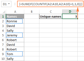
Supposing you have a column of names in your Excel worksheet, and you need to count unique names in that column. The solution is to use the SUM function in combination with IF and COUNTIF:
Note. This is an array formula, so be sure to press Ctrl + Shift + Enter to complete it. Once you do this, Excel will automatically enclose the formula in {curly braces} like in the screenshot below. In no case should you type the curly braces manually, that won't work.
In this example, we are counting unique names in range A2:A10, so our formula takes the following shape:
=SUM(IF(COUNTIF(A2:A10,A2:A10)=1,1,0))
Further on in this tutorial, we are going to discuss a handful of other formulas to count unique values of different types. And because all those formulas are variations of the basic Excel unique values formula, it makes sense to break down the above formula, so you can fully understand how it works and tweak it for your data. If someone is not interested in technicalities, you can skip right to the next formula example.
How the Excel count unique values formula works
As you see, 3 different functions are used in our unique values formula - SUM, IF and COUNTIF. Looking from the inside out, here's what each function does:
- The COUNTIF function counts how many times each individual value appears in the specified range.
In this example,
COUNTIF(A2:A10,A2:A10)returns the array{1;2;2;1;2;2;2;1;2}. - The IF function evaluates each value in the array returned by COUNTIF, keeps all 1's (unique values), and replaces all other values with zeros.
So, the function
IF(COUNTIF(A2:A10,A2:A10)=1,1,0)becomesIF(1;2;2;1;2;2;2;1;2) = 1,1,0,which turns into the array{1;0;0;1;0;0;0;1;0}where 1 is a unique value and 0 is a duplicate value. - Finally, the SUM function adds up the values in the array returned by IF and outputs the total number of unique values, which is exactly what we wanted.
Tip. To see what a specific part of your Excel unique values formula evaluates to, select that part in the formula bar and press the F9 key.
Count unique text values in Excel
If your Excel list contains both numerical and text values, and you want to count only unique text values, add the ISTEXT function to the array formula discussed above:
=SUM(IF(ISTEXT(A2:A10)*COUNTIF(A2:A10,A2:A10)=1,1,0))
As you know, the Excel ISTEXT function returns TRUE if an evaluated value is text, FALSE otherwise. Since the asterisk (*) works as the AND operator in array formulas, the IF function returns 1 only if a value is both text and unique, 0 otherwise. And after the SUM function adds up all 1's, you will get a count of unique text values in the specified range.
Don't forget to press Ctrl + Shift + Enter to correctly enter the array formula, and you will get a result similar to this:
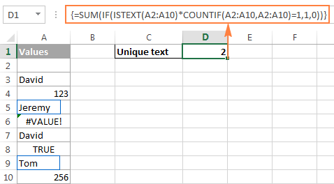
As you can see in the screenshot above, the formula returns the total number of unique text values, excluding blank cells, numbers, logical values of TRUE and FALSE, and errors.
Count unique numeric values in Excel
To count unique numbers in a list of data, utilize an array formula like we've just used for counting unique text values, with the only difference that you embed ISNUMBER instead of ISTEXT in your unique values formula:
=SUM(IF(ISNUMBER(A2:A10)*COUNTIF(A2:A10,A2:A10)=1,1,0))
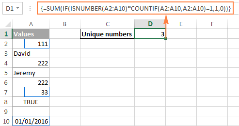
Note. Since Microsoft Excel stores dates and times as serial numbers, they are also counted.
Count case-sensitive unique values in Excel
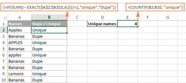
If your table contains case-sensitive data, the easiest way to count unique values would be creating a helper column with the following array formula to identify duplicate and unique items:
=IF(SUM((--EXACT($A$2:$A$10,A2)))=1,"Unique","Dupe")
And then, use a simple COUNTIF function to count unique values:
=COUNTIF(B2:B10, "unique")
Count distinct values in Excel (unique and 1st duplicate occurrences)
To get a count of distinct values in a list, use the following formula:
Remember, it's an array formula, and therefore you should press the Ctrl + Shift + Enter shortcut instead of the usual Enter keystroke.
Alternatively, you can use the SUMPRODUCT function and complete the formula in the usual way by pressing the Enter key:
For example, to count the distinct values in range A2:A10, you can go with either:
=SUM(1/COUNTIF(A2:A10,A2:A10))
Or
=SUMPRODUCT(1/COUNTIF(A2:A10,A2:A10))
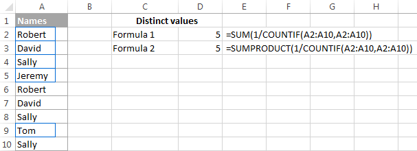
How the Excel distinct formula works
As you already know, we use the COUNTIF function to find out how many times each individual value appears in the specified range. In the above example, the result of the COUNTIF function is the following array: {2;2;3;1;2;2;3;1;3}.
After that, a number of division operations are performed, where each value of the array is used as a divisor with 1 as the dividend. This turns all duplicates values into fractional numbers corresponding to the number of duplicate occurrences. For example, if a value appears 2 times in the list, it generates 2 items in the array with a value of 0.5 (1/2=0.5). And if a value appears 3 times, it produces 3 items in the array with a value of 0.3(3). In our example, the result of 1/COUNTIF(A2:A10,A2:A10)) is the array {0.5;0.5;0.3(3);1;0.5;0.5;0.3(3);1;0.3(3)}.
Doesn't make much sense so far? That's because we haven't applied the SUM / SUMPRODUCT function yet. When one of these functions adds up the values in the array, the sum of all fractional numbers for each individual item always yields 1, no matter how many occurrences of that item exist in the list. And because all unique values appear in the array as 1's (1/1=1), the final result returned by the formula is the total number of all different values in the list.
Formulas to count distinct values of different types
As is the case with counting unique values in Excel, you can use variations of the basic Excel count distinct formula to handle specific value types such as numbers, text, and case-sensitive values.
Please remember that all of the below formulas are array formulas and require pressing Ctrl + Shift + Enter.
Count distinct values ignoring empty cells
If a column where you want to count distinct values might contain blank cells, you should add an IF function that will check the specified range for blanks (the basic Excel distinct formula discussed above would return the #DIV/0 error in this case):
For example, to count distinct values in range A2:A10, use the following array formula:
=SUM(IF(A2:A10<>"",1/COUNTIF(A2:A10, A2:A10), 0))

Formula to count distinct text values
To count distinct text values in a column, we'll be using the same approach that we've just used to exclude empty cells.
As you can easily guess, we will simply embed the ISTEXT function into our Excel count distinct formula:
And here's a real-life formula example:
=SUM(IF(ISTEXT(A2:A10),1/COUNTIF(A2:A10, A2:A10),""))
Formula to count distinct numbers
To count distinct numeric values (numbers, dates and times), use the ISNUMBER function:
For example, to count all different numbers in range A2:A10, use the following formula:
=SUM(IF(ISNUMBER(A2:A10),1/COUNTIF(A2:A10, A2:A10),""))
Count case-sensitive distinct values in Excel
Similarly to counting case-sensitive unique values, the easiest way to count case-sensitive distinct values is to add a helper column with the array formula that identifies unique values including first duplicate occurrences. The formula is basically the same as the one we used to count case-sensitive unique values, with one small change in a cell reference that makes a great difference:
=IF(SUM((--EXACT($A$2:$A2,$A2)))=1,"Distinct","")
As you remember, all array formulas in Excel require pressing Ctrl + Shift + Enter.
After the above formula is finished, you can count "distinct" values with a usual COUNTIF formula like this:
=COUNTIF(B2:B10, "distinct")
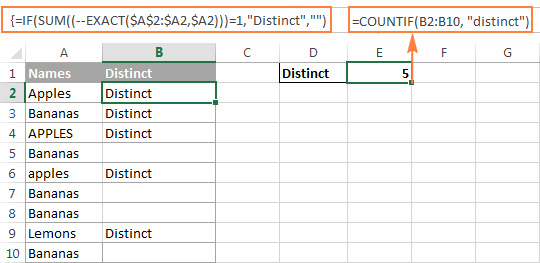
If there is no way you can add a helper column to your worksheet, you can use the following complex array formula to count case-sensitive distinct values without creating an additional column:
=SUM(IFERROR(1/IF($A$2:$A$10<>"", FREQUENCY(IF(EXACT($A$2:$A$10, TRANSPOSE($A$2:$A$10)), MATCH(ROW($A$2:$A$10), ROW($A$2:$A$10)), ""), MATCH(ROW($A$2:$A$10), ROW($A$2:$A$10))), 0), 0))
Count unique and distinct rows in Excel
Counting unique / distinct rows in Excel is akin to counting unique and distinct values, with the only difference that you use the COUNTIFS function instead of COUNTIF, which lets you specify several columns to check for unique values.
For example, to count unique or distinct names based on the values in columns A (First Name) and B (Last Name), use one of the following formulas:
Formula to count unique rows:
=SUM(IF(COUNTIFS(A2:A10,A2:A10, B2:B10,B2:B10)=1,1,0))
Formula to count distinct rows:
=SUM(1/COUNTIFS(A2:A10,A2:A10,B2:B10,B2:B10))

Naturally, you are not limited to counting unique rows based only on two columns, the Excel COUNTIFS function can process up to 127 range/criteria pairs.
Count distinct values in Excel using a PivotTable
The latest versions of Excel 2013 and Excel 2016 have a special feature that allows counting distinct values automatically in a pivot table. The following screenshot gives an idea of how the Excel Distinct Count looks like:
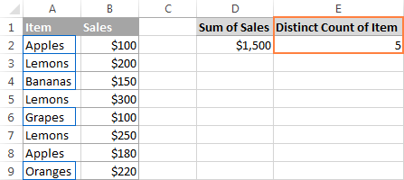
To create a pivot table with the distinct count for a certain column, perform the following steps.
- Select the data to be included in a pivot table, switch to the Insert tab, Tables group, and click the PivotTable button.
- In the Create PivotTable dialog, choose whether to place your pivot table in a new or existing worksheet, and be sure to select the Add this data to the Data Model checkbox.

- When your pivot table opens, arrange the Rows, Columns and Values areas the way you want. If you don't have much experience with Excel pivot tables, the following detailed guidelines may prove helpful: Creating a PivotTable in Excel.
- Move the field whose distinct count you want to calculate (Item field in this example) to the Values area, click on it, and select Field Value Settings… from the drop-down menu:

- The Value Field Settings dialog window will open, you scroll down to Distinct Count, which is the very last option in the list, select it and click OK.
You can also give a custom name to your Distinct Count if you want to.

Done! The newly created pivot table will display the distinct count like shown in the very first screenshot in this section.
Tip. After updating your source data, remember to update the PivotTable to bring the distinct count up to date. To refresh a pivot table, just click the Refresh button on the Analyze tab, in the Data group.
This is how you count distinct and unique values in Excel. If someone wants to have a closer look at the formulas discussed in this tutorial, you are welcome to download the sample workbook at the end of the article.
I thank you for reading and hope to see you again next week. In the next article, we are going to discuss various ways to find, filter, extract and highlights unique values in Excel. Please stay tuned!
Practice workbook for download
Excel Count Unique - formula examples (.xlsx file)
 by
by
236 comments
Good Day, I need to count unique names in a column but only the first six characters is relevant in each name. So for instance name "Sale Price" I only need for example "Sale P" so =LEFT(A2,6) but need a count of distinct occurrences such as "Sale P"; Sold; Purch. etc. ( I know some will return incomplete its not words I want but distinct occurrences.) I want to know if that column contain any sales or purchases etc. I don't want a filter with predetermined names I could have unexpected names.
Hello Phil!
If I understand your task correctly, this article may be helpful: Excel formula to count cells with certain text (exact and partial match).
For EXP
in C-I enter - RUMAITHA
in E-I enter - PKG-05
in AF-I enter - Date (But will put only when the work finish) otherwise it blank
So pls advice the formula how to calculate the common value PKG-05... once it put the date (It showing the add in the Qyt).... otherwise i did't put the date than it will not count
Hi! Please clarify your specific problem or provide any additional details to make it clear exactly what it is you need. It's difficult to tell exactly what you're asking for as it's currently written.
How would you convert your formula for DISTINCT values using CSE, ie. {=SUM(1/COUNTIF(range, range))} in Excel 365?
Hi! I'm not quite sure what you want. This formula counts distinct values. This formula and other formulas are described in detail in the paragraph above: Count distinct values in Excel (unique and 1st duplicate occurrences). Explain your question in detail.
The formula above, and the one using SUMPRODUCT, require C+S+E. Is there another way of writing these formulas using dynamic arrays ( not using C+S+E )?
Hi! If your Excel supports dynamic arrays, you don't need to use Ctrl+Shift+Enter when entering a formula. Read more about this here: Excel dynamic arrays, functions and formulas.
You can see other ways to calculate distinct values using dynamic array formulas here: How to count unique values in Excel 365. I hope it’ll be helpful.
Hi, thanks for your prompt reply. I didn't realize I could just omit the C+S+E. I tried it and it works. Thanks again.
Can you confirm the formula to count distinct text values ignoring empty cells. I should probably be able to work it out from what you've given us so far but I can't! Thanks.
Hi! Pay attention to the following paragraph of the article above: Count distinct values ignoring blank cells.
needed to count distinct values and it took a while until I found your page. You made it easy. Thank you.
Emphasize the importance of CRTL-SHIFT-ENTER, but it works great.
Hi there,
I have a report that contains multiple rows that contain the same number in Column A.
What formula would I use to get a count of unique values in Column A (i.e. exclude duplicates) that re-totals when the report is filtered on a different column (Column H in this case)?
Any tips would be appreciated :)
Steve
Hi! The Excel filter has no effect on the results of functions that count the sum or number of values, nor on the UNIQUE function.
Try to follow the recommendations from this article: Count unique values with multiple criteria.
I have a list of invoices numbers in Col F and I have the date of each invoice in Col D. I want to Write a formula that looks at Cell O4 that (Month-Year) and get a count of distinct invoices from that month. I do not want to use pivot tables becasue they take up too much storage and my file is already large.
Any help would be very apprecitaed.
Hi! You can use the information from the article above or these instructions: COUNTIF formulas for dates. Unfortunately, this information is not enough to recommend a formula to you. Which value is written in cell O4 - date or text?
If there are duplicates in column F and you want to count only unique values, use these instructions: Count unique values with criteria.
To recommend a formula, please describe the problem in detail.
Hi,
I want to count distinct value in a dynamic table.
I have applied "slicer" and want to count distinct value from visible rows of table.
Count should change as I change slicer criteria.
Thanks!
Hi! The COUNTIF function and other functions recommended in this article for counting distinct values can't ignore hidden rows.
Try to use the recommendations described in this article: How to count unique values in Excel with criteria.
always struggled with this scenario
col a col b
1 1
1 0
2 1
3 1
4 1
4 0
5 1
2 0
the question in column b is "is the value in column A unique ?" 1 for yes and 0 for no. I've only achieved this with sorting the data and then using A2=A3 true/false
Hi! The answer to your question can be found in this article: Distinct and unique values in Excel: how to find, filter, select and highlight.
=IF(COUNTIF($A$1:$A$10, $A1)=1, "Unique", "")
I have a bunch of excel files, each file contain a contact name, company name, phone number and email address. I would like to extract those information (contact name, company name, phone number and email address) from all the individual excel files sitting in a file folder and put them into one excel file called Customers under 4 headings (contact name, company name, phone number, email address).
All the information are located in the same cell locations for all the individual excel files.
Hi! Try to use the Combine Sheets Wizard to merge data from several worksheets of different files into a single Excel sheet.
The tool is included in the Ultimate Suite for Excel and can be used in a free trial to see how it works.
Column A Column B I want
1 John John
0 0 John
0 0 John
0 0 John
2 Charles Charles
0 0 Charles
0 0 Charles
0 0 Charles
When new serial starts in Column A, corresponding value in Column repeats itself. Kindly guide how?
Hi! If I understand your task correctly, the following formula should work for you:
=INDEX($B$1:B1, MATCH(LOOKUP(9999999999,$A$1:A1), $A$1:A1,0))
For more details on how to use the LOOKUP function to find the last non-empty cell in a column, read here: How to do Lookup in Excel: functions and formula examples.
I want to get the distinct count of 1st row wrt to the second row
Row1 Row2
Apples Nov
Apples Nov
Orange Nov
Banana Dec
Apples Dec
Orange Dec
Banana Dec
Now looking that in Nov there are count of different fruits are 2 and in Dec count of different fruits are 3
require formula for same
Hi! You can find the examples and detailed instructions here: Count unique values with criteria. You can try this formula:
=IFERROR(ROWS(UNIQUE(FILTER(A1:A7,B1:B7="Nov"))),0)
A B
F51 12345
F31 12346
F53 12347
F31 23456
F48 23456
F51 12345
F51 12349
F53 12347
I want this result (to show count of distinct values).
F51 = 2
F31 = 2
F53 = 1
F48 = 1
Pay attention to the following paragraph of the article above: How to count unique rows in Excel.
It covers your case completely.
looking to have all unique values in a column return a "1" the first time they show up, and every other time that name shows up return a "0"
Matt - 1
John - 1
Fred - 1
Matt - 0
Bob - 1
Fred - 0
Hi! You can find the examples and detailed instructions here: Distinct and unique values in Excel: how to find, filter, select and highlight. The formula might look like this:
=IF(COUNTIF($A$2:$A$10, $A2)=1, "1", "0")
This was a very helpful page, but I wanted to count blank cells. This seemed to work:
=SUM(IF(ISTEXT(),1/COUNTIF(, ),"")) + IF(COUNTBLANK(),1,0)
If I have a list of numbers (a column that represent the number of days receivable outstanding - column Days Outstanding), how do I have excel count the numbers in a specified range (Age Ranges) and enter the results in (Expected results)). For example
Days Outstanding Age Ranges Expected Results
35 0-20 1
53 21-40 1
60 41-60 2
5 61-80 1
75 81-100 1
100
Thanks much
Hi! Use substring sunctions to extract an interval of values from text. Count the number of values in the interval using the SUMPRODUCT function.
=SUMPRODUCT((A2:A10>--LEFT($B$2,SEARCH("-",$B$2)-1))*(A2:A10<--MID($B$2,SEARCH("-",$B$2)+1,3))) Hope this is what you need.
Column A Column B Column C
Student No. Student No BA No of occurrences
79700001 79700001 4
79700001 79700002 5
79700001 79700003 4
79700001 79700004 8
79700002 79700005 7
79700002 79700006 7
79700002 79700007
79700002 79700008
79700002 79700009
Which formula to use to count the of occurrences per student. The total to in Column C, as per example (manual)
Hi! I don't really understand what result you want to get, but try using these recommendations to calculate the values by condition: COUNTIF function in Excel - count if not blank, greater than, duplicate or unique. If this is not what you wanted, please describe the problem in more detail.
Hi
I want to use sumıf functions but my number is 20 character that's why my formula dosent work. These are the unique numbers but sumıf functions seems whole number are same
88662511009190000314 = SUMIF(Z:Z;AE3;AA:AA) = 21 :(
88662511009190000314
88662511009190000315
88662511009190000316
88662511009190000317
88662511009190000318
88662511009190000319
88662511009190000320
88662511009190000321
88662511009190000322
88662511009190000323
88662511009190000324
88662511009190000325
88662511009190000326
88662511009190000327
88662511009190000328
88662511009190000329
88662511009190000330
88662511009190000331
88662511009190000332
88662511009190000333
88662511009190000334
Hello! Unfortunately, Excel does not work with numbers longer than 15 characters.
15039819 469072
15039819 418462
15039844 616305
15039844 723803
15039844 723803
i expect result
15039819 469072 2
15039819 418462 2
15039844 616305 2
15039844 723803 2
15039844 723803 2
i have to count how many unique value in column B have for every value of column 1.
Thanks
Hi! Look for the example formulas here: Count unique values with criteria.
If I understand your task correctly, try the following formula:
=IFERROR(ROWS(UNIQUE(FILTER($B$1:$B$5,$A$1:$A$5=A1))), 0)
How do I do a unique count of products by supplier.
I have a distinct list of suppliers, and then a data summary of products used in a seperate table.
I've tried =if(table2[supplier]=a3,dcount(table2[product description],0) but it's not working??
Hi! If I understand your task correctly, this article may be helpful: How to count unique values in Excel with criteria.
Hi, how do I count the number of unique items in a column that fall between 2 dates. For example, how do I count each invoice number that falls between 1/1/22-2/1/22 . I was able to figure out how to count the number of invoices that fall within that date, but now I need to find the number of invoices that fall within that period.
Hi! To count the number of unique values by condition, use this guide: How to count unique values in Excel: with criteria, ignoring blanks. Try these formulas:
=COUNTA(UNIQUE(FILTER(A2:A10,(B2:B10>D1)*(B2:B10<D2))))
or
=IFERROR(ROWS(UNIQUE(FILTER(A2:A10,(B2:B10>D1)*(B2:B10<D2)))), 0)