The tutorial shows how to create an Excel drop down list depending on another cell by using new dynamic array functions.
Creating a simple drop down list in Excel is easy. Making a multi-level cascading drop-down has always been a challenge. The above linked tutorial describes four different approaches, each including a crazy number of steps, a bunch of different formulas, and a handful of limitations relating to multi-word entries, blank cells, etc.
That was the bad news. The good news is that those methods were designed for pre-dynamic versions of Excel. The introduction of dynamic arrays in Excel 365 has changed everything! With new dynamic array functions, creating a multiple dependent drop-down list is a matter of minutes, if not seconds. No tricks, no caveats, no nonsense. Only fast, straightforward and easy-to-follow solutions.
Notes:
- This new dynamic array way of making dropdown lists only works in Excel 365 and Excel 2021. In pre-dynamic Excel, you will have to do it the long old-fashioned way as described in Creating a dependent drop down in Excel 2019 - 2007.
- This solution is for a single row. If you want to copy your picklists down multiple rows, then follow the instructions in Dependent drop-down list for multiple rows.
How to make dynamic drop down list in Excel
This example demonstrates the general approach to creating a cascading drop down list in Excel by using the new dynamic array functions.
Supposing you have a list of fruit in column A and exporters in column B. An additional complication is that the fruit names are not grouped but scattered across the column. The goal is to put the unique fruit names in the first drop-down and depending on the user's selection show the relevant exporters in the second drop-down.
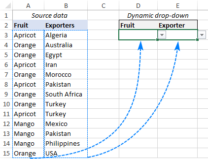
To create a dynamic dependent drop down list in Excel, carry out these steps:
1. Get items for the main drop down list
For starters, we shall extract all different fruit names from column A. This can be done by using the UNIQUE function in its simplest form - supply the fruit list for the first argument (array) and omit the remaining optional arguments as their defaults work just fine for us:
=UNIQUE(A3:A15)
The formula goes to G3, and after pressing the Enter key the results spill into the next cells automatically.

2. Create the main drop down
To make your primary drop-down list, configure an Excel Data Validation rule in this way:
- Select a cell in which you want the dropdown to appear (D3 in our case).
- On the Data tab, in the Data Tools group, click Data Validation.
- In the Data Validation dialog box, do the following:
- Under Allow, select List.
- In the Source box, enter the reference to the spill range output by the UNIQUE formula. For this, type the hash tag right after the cell reference, like this: =$G$3#
This is called a spill range reference, and this syntax refers to the entire range regardless of how much it expands or contracts.
- Click OK to close the dialog.
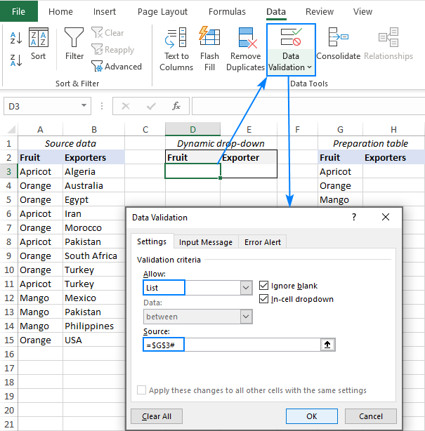
Your primary drop-down list is done!

3. Get items for the dependent drop down list
To get entries for the secondary dropdown menu, we'll filter the values in column B based on the value selected in the first dropdown. This can be done with the help of another dynamic array function called FILTER:
=FILTER(B3:B15, A3:A15=D3)
Where B3:B15 are the source data for your dependent drop down, A3:A15 are the source data for your main dropdown, and D3 is the main dropdown cell.
To make sure the formula works correctly, you can select some value in the first drop-down list and observe the results returned by FILTER. Perfect! :)

4. Make the dependent drop down
To create the second dropdown list, configure the data validation criteria exactly as you did for the first drop down at step 2. But this time, reference the spill range returned by the FILTER function: =$H$3#
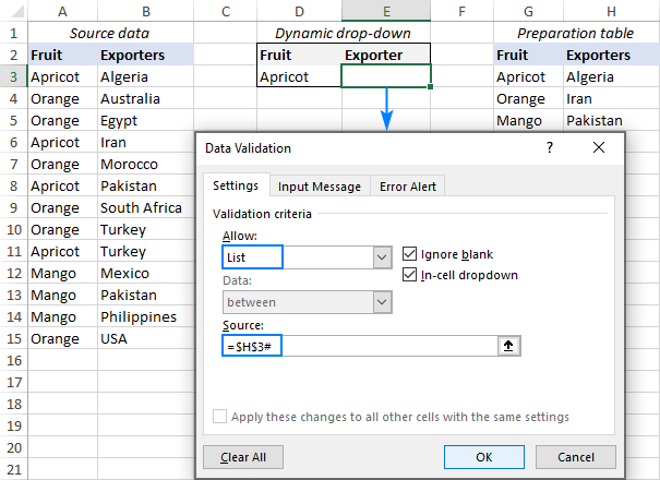
That's it! Your Excel dependent dropdown list is ready for use.

Tips and notes:
- To have the new entries included in the drop-down list automatically, format your source data as an Excel table. Or you can include a few blank cells in your formulas as demonstrated in this example.
- If your original data contains any gaps, you can filter out blanks by using this solution.
- To alphabetically sort a dropdown's items, wrap your formulas in the SORT function as explained in this example.
How to create multiple dependent drop down list in Excel
In the previous example, we made a drop down list depending on another cell. But what if you need a multi-level hierarchy, i.e. a 3rd dropdown depending in the 2nd list, or even a 4th dropdown depending on the 3rd list. Is that possible? Yes, you can set up any number of dependent lists (a reasonable number, of course :).
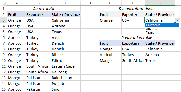
For this example, we have placed states / provinces in column C, and are now looking to add a corresponding dropdown menu in G3:

To make a multiple dependent drop down list in Excel, this is what you need to do:
1. Set up the first drop down
The main dropdown list is created with exact the same steps as in the previous example (please see steps 1 and 2 above). The only difference is the spill range reference you enter in the Source box.
This time, the UNIQUE formula is in E8, and the main drop down list is going to be in E3. So, you select E3, click Data Validation, and supply this reference: =$E$8#

2. Configure the second drop down
As you may have noticed, now column B contains multiple occurrences of the same exporters. But you want only unique names in your dropdown list, right? To leave out all duplicate occurrences, wrap the UNIQUE function around your FILTER formula, and enter this updated formula in F8:
=UNIQUE(FILTER(B3:B15, A3:A15=E3))
Where B3:B15 are the source data for the second drop down, A3:A15 are the source data for the first dropdown, and E3 is the first dropdown cell.
After that, use the following spill range reference for the Data Validation criteria: =$F$8#
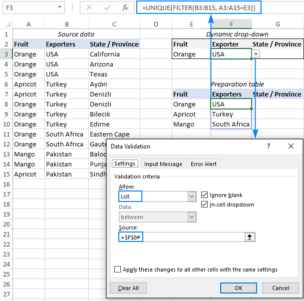
3. Set up the third drop down
To gather the items for the 3rd drop down list, make use of the FILTER formula with multiple criteria. The first criterion checks the entire fruit list against the value selected in the 1st dropdown (A3:A15=E3) while the second criterion tests the list of exporters against the selection in the 2nd dropdown (B3:B15=F3). The complete formula goes to G8:
=FILTER(C3:C15, (A3:A15=E3) * (B3:B15=F3))
If you are going to add more dependent dropdowns (4th, 5th, etc.), then most likely column C will contain multiple occurrences of the same item. To prevent duplicates from getting into the preparation table, and consequently in the 3rd dropdown, nest the FILTER formula in the UNIQUE function like we did in the previous step:
=UNIQUE(FILTER(C3:C15, (A3:A15=E3) * (B3:B15=F3)))
The last thing for you to do is to create one more Data Validation rule with this Source reference: =$G$8#

Your multiple dependent drop down list is good to go!
Tip. In a similar manner, you can get items for subsequent drop-downs. Assuming column D contains the source data for your 4th dropdown list, you can enter the following formula in H8 to retrieve the corresponding items:
=UNIQUE(FILTER(D3:D15, (A3:A15=E3) * (B3:B15=F3) * (C3:C15=G3)))
How to make an expandable drop down list in Excel
After creating a dropdown, your first concern may be as to what happens when you add new items to the source data. Will the dropdown list update automatically? If your original data is formatted as Excel table, then yes, a dynamic drop down list discussed in the previous examples will expand automatically without any effort on your side because Excel tables are expandable by their nature.
If for some reason using an Excel table is not an option, you can make your dropdown list expandable in this way:
- To include new data automatically as it is added to the source list, add a few extra cells to the arrays referenced in your formulas.
- To exclude blank cells, configure the formulas to ignore empty cells until they get filled.
Keeping these two points in mind, let's fine-tune the formulas in our data preparation table. The Data Validation rules do not require any adjustments at all.
Formula for the main dropdown
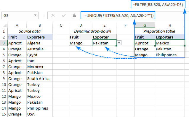
With the fruit names in A3:A15, we add 5 extra cells to the array to cater for possible new entries. Additionally, we embed the FILTER function into UNIQUE to extract unique values without blanks.
Given the above, the formula in G3 takes this shape:
=UNIQUE(FILTER(A3:A20, A3:A20<>""))
Formula for the dependent dropdown
The formula in G3 does not need much tweaking - just extend the arrays with a few more cells:
=FILTER(B3:B20, A3:A20=D3)
The result is a fully dynamic expandable dependent drop down list:
How to sort drop down list alphabetically
Want to arrange your dropdown list alphabetically without resorting the source data? The new dynamic Excel has a special function for this too! In your data preparation table, simply wrap the SORT function around your existing formulas.
The data validation rules are configured exactly as described in the previous examples.
To sort from A to Z
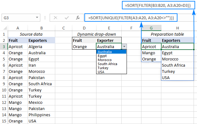
Since the ascending sort order is the default option, you can just nest your existing formulas in the array argument of SORT, omitting all other arguments which are optional.
For the main dropdown (the formula in G3):
=SORT(UNIQUE(FILTER(A3:A20, A3:A20<>"")))
For the dependent dropdown (the formula in H3):
=SORT(FILTER(B3:B20, A3:A20=D3))
Done! Both drop down lists get sorted alphabetically A to Z.
To sort from Z to A
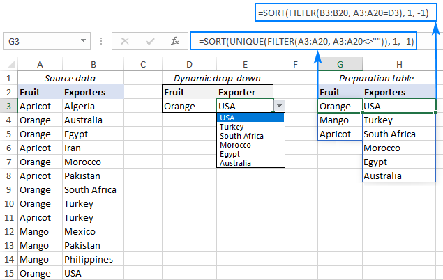
To sort in descending order, you need to set the 3rd argument (sort_order) of the SORT function to -1.
For the main dropdown (the formula in G3):
=SORT(UNIQUE(FILTER(A3:A20, A3:A20<>"")), 1, -1)
For the dependent dropdown (the formula in H3):
=SORT(FILTER(B3:B20, A3:A20=D3), 1, -1)
This will sort both the data in the preparation table and the items in the dropdown lists from Z to A:
Tip. Another fast and easy way to enter information in Excel spreadsheets is a data entry form.
That's how to create dynamic drop down list in Excel with the help of the new dynamic array functions. Unlike the traditional methods, this approach works perfectly for single and multi-word entries and takes care of any blank cells. Thank you for reading and hope to see you on our blog next week!
Practice workbook for download
Excel dependent drop down list (.xlsx file)
 by
by
166 comments
Type this in the Source for the dependent list:
=INDIRECT("TableName["&A2&"]")
Hello, for some reason the formula with a # ( =$H$3#) sign does not work on Excel for Mac in the 16.78.3 (2023), can you please recommend an alternative approach?
Hello Artem!
The formula =$H$3# might not work in Excel for Mac version 16.78.3 (2023) for several reasons:
1. Cell Formatting: Ensure the cell where you're entering the formula is set to a number or general format, not text.
2. Calculation Settings: Check if the calculation mode is set to "Automatic" under Excel -> Preferences -> Calculation.
3. Check if there is an error in cell H3, e.g. #SPILL error. Read more: Spill range reference.
4. Macro Security Settings: If the formula involves macros, ensure macros are enabled under Excel -> Preferences -> Security & Privacy -> Macro Security.
Hi, I am trying to use a drop down to automatically create a related sequential reference. For example, if I choose Leeds from the drop down, I would like a reference LS0001, LS0002, LS0003...the next in the sequence, to appear in a cell. in the next row down, if I select Manchester from the drop down I would like a reference MN0001, MN0002 etc to appear. Is this possible?
The result would look like
Leeds LS0001
Leeds LS0002
Manchester MN0001
Leeds LS0003
Manchester MN0002
Thanks for your help!
Hello Katherine!
A drop-down list can only put the value you have selected into a cell. You can replace this value with another one using VBA code.
To enter a related reference in a neighboring cell, you can use a dependent drop-down list as described in the article above. But with Excel formula you cannot automatically create its values.
You can get the desired value in a neighboring cell by combining the VLOOKUP formula, which will find the corresponding short name for the value in the neighboring cell. You can get the number 1, 2, 3 and so on using duplicate counting as described in this article: How to count duplicates in Excel.
You can write this number in the desired format using the TEXT function.
For example:
=VLOOKUP(A2,E2:F10,2)&TEXT(COUNTIF($A$2:A2,A2),"0000")
I have multiple Vendors in Column A and Account associated with Vendor in Column B. How do I create a dropdown based if I selected a Vendor from Column A and only gives me choices that is associated with that Vendor in Column B. In the example below, I would select the Vendor - Puget Sound and in Column B - it should only give me the option to pick Electricity or Gas.
e.g
Vendor Account
Puget Sound Electricity
Puget Sound Gas
Verizon Internet
SRP Electricity
Republic Trash
Hello Maggie!
All the necessary information is in the article above.
You can also find useful information in these articles: Making a dependent (cascading) drop down list in Excel and Set up dependent drop-down list for multiple rows in Excel.
Hi.
Is there any way to auto populate a dynamic dependent dropdown list if there's only one value available?
Hi! Excel does not have a standard way of automatically populating a cell with a value from a drop down list. However, you can try to do this using a VBA macro.
what an amazing explanation, big thanks for huge efforts. I add another multiple rows by making more than one unique tables
Thank You!,
Is there a way to clear the selected items once I've changed the dependent?
Again Thank You!!!!!!!!
Hi! You can clear the selected items in a cell by editing cell and pressing DEL key.
Hi,
What happens if you have multiple dynamic dropdowns,
Many rows where you choose different fruits and then need the exporters available in column E
D3 has Apricot and the choices are available as expected in E3 - data comes from $F$8#
D4 has Orange but the choices available in E4, are still for Apricot, as the Exporter list is still referring to the Fruit in D3. $F$8#
Hi! Try carefully using the instructions in the third section of this article: How to make an expandable dropdown list in Excel.
I think you didn't get the question.
They have a column to apply the validation, not only one row.
It does not work because the FILTER refers only to a one single cell.
If they enter Apricot in D3, the list available for E3 is good
Then, they entered Orange in D4, the list in E4 is the list for Apricot, instead of list for Orange
Based on this description, it is hard to completely understand the task. However, I’ll try to guess and offer the following guide: Making a dependent (cascading) drop down list in Excel.
Hi, the question the user is asking is how do we handle multiple rows in the output/dropdown section. Your example currently only has one row D3 & E3. What happens if we add a second row? D4 & E4. Do we need to have a formula for each row?
I have exactly the same question. I want to use the dynamic dropdowns to choose values for multiple rows, not just one row. But you are using the chosen value of a specific cell (D3) as filter for the items for the dependent drop down list in E3. What if I now choose a different value in D4, and in E4 want to see the dependent dropdown for the chosen value in D4, do I need to create a new list? And link the E4 dropdown to that list? That is becoming unpractical if I need to do this for multiple rows, because each row would need its own dependent drop down list, based on the value chosen in column D for that row...
I should have clarified that it will not work since you will get a spill over error in the next row.
Hello Rob!
Maybe this article will be helpful: Spill in Excel - tutorial with examples.
If columns D and E were a multi-row table, this solution does not work.
Hello Rob!
If I understand you correctly, your table has several values in one cell. A dependent drop-down list cannot work for multiple values at once.
However, maybe you will find this article useful: Dependent drop down list for multiple rows using Excel dynamic arrays.
for the preparation table add transpose : =TRANSPOSE(UNIQUE(FILTER($B$3:$B$15, $A$3:$A$15=G3)))
Then it spills horizontally.
Then you can drag down for multiple entries.
For the validation: take out the $ before the row number to drag down different drop down lists.
Hi! A dropdown list in Excel works for only one cell. You can copy dropdown list to another cell as described in these instructions: How to edit, copy and delete drop down list in Excel.
Hi! A drop-down list is a tool for validating the data that is entered into a cell. Therefore, it is created for each cell separately. Please take a look at this guide: How to copy drop down list in Excel.
To use the Filter function but it links to another worksheet
Hi! You can use an external reference to another worksheet in the FILTER function. Suppose you have data in Sheet2 (A1:B10) and want to filter rows where the value in column A is greater than 50. You can use the following formula in a cell on your current sheet:
=FILTER(Sheet2!A1:B10, Sheet2!A1:A10>50)
I recommend reading this guide: Excel reference to another sheet or workbook (external reference).
Thank you, but my excel is in new version and it does not have filter and unique formula, can you please help?
Hi! The FILTER function is available in Excel for Microsoft 365, Excel 2021, Excel 2019. The UNIQUE function is available in Excel for Microsoft 365, Excel 2021.
Hello,
I have question about first section : How to make dynamic drop down list in Excel.
D3 is your main dropdown cell. What if i want to have dropdown cell in another rows (D4, D5.... ) with same filter options and sorce data?
Thank you
Hi! You can find the answer to your question in this article: How to copy drop down list in Excel.
Hi! The quoted article explains how to extend the main dropdown to further rows. Is there a way to do the same with the dependent dropdown?
That is, with the example of this article, make every cell in the E column have a dropdown that depends on the value of the cell in the D column of the corresponding row.
Thank you
Hi! You can make a dynamic dependent dropdown list yourself by using these instructions: Set up dependent drop-down list for multiple rows in Excel.
Hello, I have a list of 5 criteria questions that will be selected and based on those answer I want to feedback to be the top 3 choices based on the questions the selected. How would I write the formula, I am thinking we will need to assign a value on the answer they selected before selecting the top 3 options to select from
Hi! Please clarify your specific problem or provide additional details to highlight exactly what you need. As it's currently written, it's hard to tell exactly what you're asking.
Thank you for this! This was very helpful and worked in my first three drop down. We could finally automate our reports. However, I have 4 drop down that needs to be made. What would be the formula if I need 4 drop down? Thank you.
Hi! The code works for all drop-down lists on your worksheet. Unless you specify a range of cells in which it can work. This is explained in the article above.
I followed these steps almost excatly and was so excited I finally found a way to get my drop dowans to work I got the first 2 drop downs to work but then I keep getting a calc error on the third -.-.
Source Data Table:
Column 1 = A1000 - A1329
Column 2 = B1000 - B1329
Column 3 = C1000 - C1329
Prep Table:
First drop down in cell F1000 reads - =UNIQUE(A1000:A1329)
Second drop down in cell G1000 reads =UNIQUE(FILTER(B1000:B1329,A1000:A1329=L1000)
Third drop down, dysplaying #CALC!, in cell H000 reads =UNIQUE(FILTER(C1000:C1329,(A1000:A1329=L1000)*(B1000:B1329=M1000)))
Dynamic Table:
Cell L1000 drop down works (data validation reads =$F$1000#)
Cell M1000 drop down works (data validation reads =$G$1000#)
Cell N1000 drop down does not work and displays the #CALC! error (data validation reads =$H$1000#)
Im not sure if you can help provide all these details but im not sure what im doing wrong.
Hopefully someone can help, thank you in advance this guide is great!
Hi! Sorry, I can't recommend a formula to you as I can't see your data.
I am trying to create a drop down of product names, but each name has three or four specific fields of dependent data to that product name that I want to come over as it is selected from the drop down. Once an item is selected from the drop down, a calculator will reference that data to come up with a specific number. Is that possible?
Hi! A drop-down list creates a standard text string. No references or data fields are possible. With the selected value, you can then use a formula to retrieve the data associated with it. For example, using VLOOKUP or INDEX+MATCH. I hope I've understood what you're asking.
Is there a way to be able to use our dynamic lists for each row?
Basically what I am wanting to do is the Value of cells in Column D depend on value selected in Column C - for each row.
Hi! All the necessary information is in the article above.
Hello!
Say I am tracking equipment on a large construction project that includes 4 different construction sites where equipment will be either stored or utilized. Each construction site will have its own area on an excel sheet (all 4 on the same sheet for better visualization when determining equipment needs). Using source data, I create 4 identical lists of available equipment for the project, one for each site. Is it possible to have parameters in each list such that when I select a piece of equipment that is currently in site #1, that same piece of equipment would not be show up in the same list in site #2 (or site #3 and #4, for that matter) for selection, until that piece of equipment is de-selected? I hope that makes sense! My main concern is eliminating the potential of showing the same piece of equipment in two different sites. Thank you!
Hi! You're asking beyond the advice this blog can provide. Solving this complex problem requires more than a single formula. If you have a specific question about how a function or a formula works, I'll do my best to help you.
Hi Sir,
I have three dependent values similar to Fruit, Exporters and State/Province. In the above example, there are 3 sections like the Source data, preparation table and the Dynamic drop-down area. in the Dynamic drop-down area, currently only one row and their drop-down results are shown. I have a scenario where the Dynamic drop-down is there in a separate sheet and I have to do it for multiple rows. i.e., In Row 1, User would select Orange, USA and the State list will be shown. in the Row 2 and subsequent rows, select the Fruit and Exporter, based on it show the third drop-down list for multiple rows.
Hi! If I understand the question correctly, you can create dependent dropdown lists as described in this guide. But without seeing your data, it is impossible to offer you formulas for this.
Is it possible to make the pulled data editable? When I change this data it disappears. Thank you!
Hi! If you select a new value from the drop-down list, the old value disappears and is replaced by the new value. If you want to select multiple values from the drop-down list, visit: How to make Excel drop down list with multiple selections.
Thanks, learned something new today :)