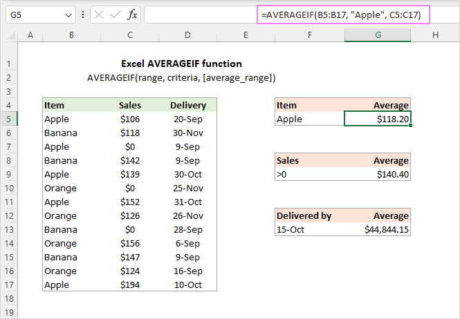
The tutorial shows how to use the AVERAGEIF function in Excel to calculate an arithmetic mean with condition.
Microsoft Excel has a few different functions to calculate an arithmetic mean of numbers. When you are looking to average cells that meet a certain condition, AVERAGEIF is the function to use.
AVERAGEIF function in Excel
The AVERAGEIF function is used to calculate an average of all cells in a given range that meet a certain condition.
The function has a total of 3 arguments - the first 2 are required, the last one is optional:
- Range (required) - the range of cells to test against the criteria.
- Criteria (required)- the condition that determines which cells to average. It can be supplied in the form of a number, logical expression, text value, or cell reference, e.g. 5, ">5", "cat", or A2.
- Average_range (optional) - the cells you actually want to average. If omitted, then range will be averaged.
The AVERAGEIF function is available in Excel 365 - 2007.

Tip. To average cells with two or more criteria, use the AVERAGEIFS function.
Excel AVERAGEIF - things to remember!
To efficiently use the AVERAGEIF function in your worksheets, take notice of these key points:
- When calculating an average, empty cells, text values, and logical values TRUE and FALSE are ignored.
- Zero values are included in the average.
- If a criteria cell is empty, it is treated as a zero value (0).
- If average_range contains only blank cells or text values, a #DIV/0! error occurs.
- If no cell in range meets criteria, a #DIV/0! error is returned.
- The Average_range argument does not necessarily have to be of the same size as range. However, the actual cells to be averaged are determined by the size of the range argument. In other words, the upper left cell in average_range becomes the starting point, and as many columns and rows are averaged as contained in the range argument.
AVERAGEIF formula based on another cell
With the Excel AVERAGEIF function, you can average a column of numbers based on:
- criteria applied to the same column
- criteria applied to another column
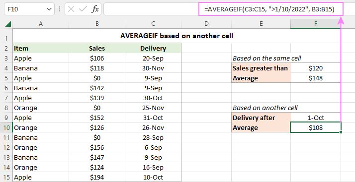
In case the condition applies to the same column that should be averaged, you define only the first two arguments: range and criteria. For example, to find an average of sales in B3:B15 that are greater than $120, the formula is:
=AVERAGEIF(B3:B15, ">120")
To average based on another cell, you define all 3 arguments: range (cells to check against the condition), criteria (the condition) and average_range (cells to calculate).
For instance, to get an average of sales that were delivered after Oct-1, the formula is:
=AVERAGEIF(C3:C15, ">1/10/2022", B3:B15)
Where C3:C15 are the cells to check against the criteria and B3:B15 are the cells to average.

How to use AVERAGEIF function in Excel - examples
And now, let's see how you can use Excel AVERAGEIF in real-life worksheets to find an average of cells that meet your criteria.
AVERAGEIF text criteria
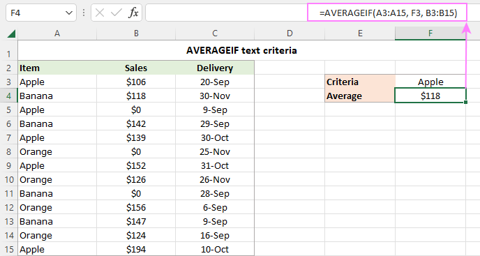
To find an average of numeric values in a given column if another column contains certain text, you build an AVERAGEIF formula with text criteria. When a text value is included directly in the formula, it should be enclosed in double quotes ("").
For example, to average the numbers in column B if column A contains "Apple", the formula is:
=AVERAGEIF(A3:A15, "apple", B3:B15)
Alternatively, you can input the target text in some cell, say F3, and use that cell reference for criteria. In this case, double quotes are not needed.
=AVERAGEIF(A3:A15, F3, B3:B15)
The advantage of this approach is that it lets you average sales for any other item by simply changing the text criteria in F3, without having to make any adjustments to the formula.

Tip. To round an average to a certain number of decimal places, make use of the Increase Decimal or Decrease Decimal command on the Home tab, in the Number group. This will change the display representation of the average but not the value itself. To round the actual value returned by the formula, use AVERAGEIF together with ROUND or other rounding functions. For more information, please see How to round average in Excel.
AVERAGEIF logical criteria for numeric values
To test various numeric values in your criteria, use them together with "greater than" (>), "less than" (<), equal to (=), not equal to (<>), and other logical operators.
When including a logical operator with a number, remember to enclose the whole construction in double quotes. For example, to average the numbers that are less than or equal to 120, the formula would be:
=AVERAGEIF(B3:B15, "<=120")
Pay attention that the operator and number are both enclosed in quotes.
When using the "is equal to" criteria, the equality sign (=) can be omitted.
For instance, to average the sales delivered on 9-Sep-2022, the formula goes as follows:
=AVERAGEIF(C3:C15, "9/9/2022", B3:B15)

Using AVERAGEIF with dates
Similar to numbers, you can use dates as criteria for the AVERAGEIF function. Date criteria can be constructed in a few different ways.
Let's take a look at how you can average sales delivered before a given date, say November 1, 2022.
The easiest way is to enclose the logical operator and date together in double quotes:
=AVERAGEIF(C3:C15, "<11/1/2022", B3:B15)
Or you can enclose the operator and the date in quotes separately and concatenate them using the & sign:
=AVERAGEIF(C3:C15, "<"&"11/1/2022", B3:B15)
To make sure the date is entered in the format that Excel understands, you can use the DATE function concatenated with the logical operator:
=AVERAGEIF(C3:C15, "<"&DATE(2022, 11, 1), B3:B15)
To average sales delivered by today's date, use the TODAY function in the criteria:
=AVERAGEIF(C3:C15, "<"&TODAY(), B3:B15)
The screenshot below shows the results:

AVERAGEIF greater than 0
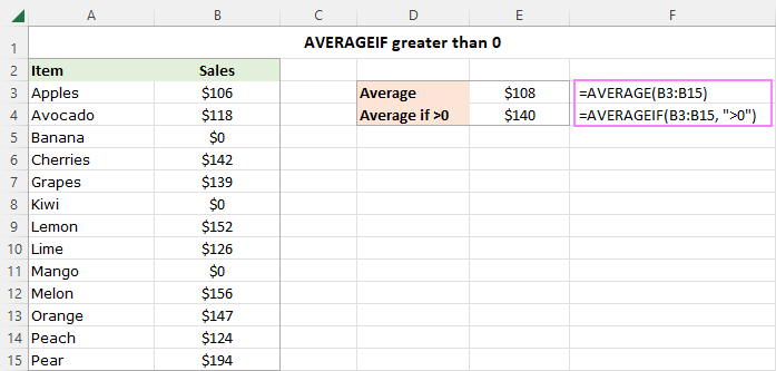
By design, the Excel AVERAGE function skips blank cells but includes 0 values in calculations. To only average values greater than zero, use ">0" for criteria.
For example, to calculate an average of the numbers in B3:B15 that are greater than zero, the formula in E4 is:
=AVERAGEIF(B3:B15, ">0")
Please notice how the result differs from a normal average in E3:

Average if not 0
The above solution works nicely for a set of positive numbers. If you have both positive and negative values, then you can average all numbers excluding zeros using "<>0" for criteria.
For instance, to average all the values in B3:B15 except zeros, use this formula:
=AVERAGEIF(B3:B15, "<>0")

Excel average if not zero or blank
As the AVERAGEIF function skips empty cells by design, you can simply use the "not zero" criteria ("<>0"). As a result, both zero values and blank cells will be ignored. To make sure of this, in our sample data set, we replaced a couple of zero values with blanks, and got absolutely the same result as in the previous example:
=AVERAGEIF(B3:B15, "<>0")

Average if another cell is blank
To average cells in a given column if a cell in another column in the same row is blank, use "=" for criteria. This will include empty cells that contain absolutely nothing - no space, no zero-length string, no non-printing characters, etc.
To average values corresponding to visually blank cells including those that contain empty strings ("") returned by other functions, use "" for criteria.
For testing purposes, we will use both criteria to average the numbers in B3:B15 that have no delivery date in C3:C15 (i.e. if a cell in column C is blank).
=AVERAGEIF(C3:C15, "=", B3:B15)
=AVERAGEIF(C3:C15, "", B3:B15)
Because one of the visually blank cells (C12) is not really empty - there is a zero-length string in it - the formulas deliver different results:

Average if another cell is not blank
To average a range of cells if a cell in another range is not blank, utilize "<>" for criteria.
For instance, the following AVERAGEIF formula calculates an average of cells B3 through B15 if a cell in column C in the same row is not blank:
=AVERAGEIF(C3:C15, "<>", B3:B15)

AVERAGEIF wildcard (partial match)
To average cells based on partial match, use wildcard characters in the criteria of your AVERAGEIF formula:
- A question mark (?) to match any single character.
- An asterisk (*) to match any sequence of characters.
Suppose you have 3 different sorts of banana, and you want to find their average. The following formula will make it happen:
=AVERAGEIF(A3:A15, "*banana", B3:B15)
If needed, a wildcard character can be used together with a cell reference. Assuming the target item is in cell В4, the formula takes this shape:
=AVERAGEIF(A3:A15, "*"&D4, B3:B15)

If your keyword may appear anywhere in a cell (in the beginning, in the middle, or in the end), place an asterisk on both sides:
=AVERAGEIF(A3:A15, "*banana*", B3:B15)
To find the average of all items excluding any banana, use this formula:
=AVERAGEIF(A3:A15, "<>*banana*", B3:B15)
How to calculate average in Excel excluding certain cells
To exclude certain cells from the average, use the "not equal to" (<>) logical operator.
For example, to average the sales numbers for all the items except "apple", use this formula:
=AVERAGEIF(A3:A15, "<>apple", B3:B15)
If the excluded item is in a predefined cell (D4), the formula takes this form:
=AVERAGEIF(A3:A15, "<>"&D4, B3:B15)
To find the average of all items excluding any "banana", use the "not equal to" together with a wildcard:
=AVERAGEIF(A3:A15, "<>*banana", B3:B15)
In case the excluded wildcard item is in a separate cell (D9), then concatenate the logical operator, wildcard character and cell reference using an ampersand:
=AVERAGEIF(A3:A15,"<>"&"*"&D9, B3:B15)

How to use AVERAGEIF with cell reference
Instead of typing the criteria directly in a formula, you can use a logical operator in combination with a cell reference to construct the criteria. This way, you will be able to test different conditions by changing a value in the criteria cell without editing your AVERAGEIF formula.
When the condition defaults to "is equal to", you simply use a cell reference for the criteria argument. The below formula calculates the average of all sales within the range B3:B15 relating to the item in cell F4.
=AVERAGEIF(A3:A15, F4, B3:B15)
When the criteria includes a logical operator, you build it in this way: enclose the logical operator in quotation marks and use an ampersand (&) to concatenate it with a cell reference.
For example, to find the average of sales in B3:B15 that are greater than the value in F9, use the following formula:
=AVERAGEIF(B3:B15, ">"&F9)
In a similar fashion, you can use a logical expression with another function in the criteria.
With dates in C3:C15, the below formula returns the average of sales that have been delivered up to the current date inclusive:
=AVERAGEIF(C3:C15, "<="&TODAY(), B3:B15)

That's how you use the AVERAGEIF function in Excel to calculate an arithmetic mean with condition. I thank you for reading and hope to see you on our blog next week!
Practice workbook for download
Excel AVERAGEIF function - examples (.xlsx file)
 by
by
46 comments
Is there a way to average cells with the < symbol in the cell. Example A1 is <.10 A2 is <.10 A3 is .11 and A4 is .12 How would I get the average of those 4 cells?
Hello Robert!
Your cells contain text. Using the MID function and a math operation, extract the digits from the text and convert them to numbers. Read more: How to convert text to number in Excel.
You can then calculate the average value.
=AVERAGE(--MID(A1:A4,2,10))
Hello, thank you for the post. I am trying top get average of multiple IDs at the same time and I have around 1400 Ids. Do I have to calculate them separately? I mean I have apple, banana, berry, pear.. .. how can I calculate all at once?
Hello! If you want to calculate the average value when several conditions are met at once, use the AVERAGEIFS function and these instructions: Excel AVERAGEIFS function with multiple criteria.
Can I average of greater than 0 less than 25
Please re-check the article above since it covers your case.
Hi,
hoping to get help,
i want to get the average for a multiple criteria but it is returning error as i have negative numbers, how can i do the calculation including the negative value without returning error result.
thanks in advance
Hi! AVERAGE and AVERAGEIF functions also work with negative numbers. Therefore, this is not the cause of the error. Describe your task in more detail. Please specify what you were trying to find, what formula you used, and what problem or error occurred. Give an example of the source data and the expected result.
Hi
Thanks for all the very useful tutorials and tricks to be found here in your blog. It's really helpful to me.
I am using the following averageif formula to get the average of the last four cells and so far it works fine:
=IFERROR(AVERAGEIF((OFFSET(D6;0;COUNT(E6:BF6);1;-4));">0";OFFSET(D6;0;COUNT(E6:BF6);1;-4));0)
Question: how can I extend the formula in not considering the cell with the highest value in the average calculation ("cut peak value"). I tried it with MAX but I was not able to extend the formula correctly.
Example: 4 cells showing value - 10 / 10 / 50 / 10 ==> deduct the 50 and give me back the average of the remaining values (in this case 10).
Many thanks.
Regards, andi
Example:
Hi! If my understanding is correct, the following formula should work for you:
=AVERAGE(IF(MAX(OFFSET(D6,0,COUNT(E6:BF6),1,-4)) = OFFSET(D6,0,COUNT(E6:BF6),1,-4), "", OFFSET(D6,0,COUNT(E6:BF6),1,-4)))
Awesome, exactly what I was looking for. Thanks a lot for your swift reply, very much appreciated. BR, andi
Hi,
Is it possible to do it with a conditional? For example the average of all the apples sold after certain date?
Hi! If you want to calculate the average of two or more conditions, use these instructions: Excel AVERAGEIFS function with multiple criteria. It's also written in the article above.
Hi, I want to use Averageif with a function for my criteria, isnumber. I ask students to mark each other's groups, but they write all kinds of random text when it's their own group, they don't just leave it blank. I've tried AVERAGEIF(I1:I29;"IFNUMBER") and I'm getting divide by zero.
Hi! Your task is not completely clear to me. Unfortunately, without seeing your data it is difficult to give you any advice. Please provide me with an example of the source data and the expected result. Also note the syntax of the AVERAGEIF function, as you are doing it incorrectly.
Hello Alexander,
I have a problem which I tried to resolve through conditional formatting tool yet with no success.
I have two sets of data on the same spreadsheet. First dataset (e.g., B2:M101) - monthly precipitation, with 12 columns (= months from Jan to Dec). Second adjacent dataset (N2:Y101) - monthly temperatures, also with 12 columns (=months). Rows are geographic locations, same for both datasets. Hence, the overall design is that for each location (row) I have monthly prec. and temp. data.
The task is to calculate, within each location (row), an average temperature of three consecutive months (a quarter) with the highest cumulative precipitation.
Firstly, I identify three adjacent cells in a row in the first dataset (precipitation) which make the highest value when summed. I can get this value for the first row by using an array formula =MAX(B2:K2+C2:L2+D2:M2) (followed by pressing Ctrl+Shift+Enter), and then manually check which exact cells make this value (these will constitute the wettest quarter). Let's say, these cells are B2, C2 and D2 making up a quarter Jan-Feb-Mar.
Secondly, I have to calculate average of the corresponding three cells (Jan-Feb-Mar) in the second dataset (temperature), which are in the same row.
Question: is there any function (algorithm) in Excel allowing to perform this sort of calculation, i.e., find an average of a group of cells based on the sum of another group of cells in the same row? I tried AVERAGEIF function, using the above array formula as a condition, but it didn't work. Could you please suggest any algorithm that would make such calculation fast? The entire dataset includes some thousands of rows, hence manual calculation of each row is quite a lot of work.
Would appreciate any help.
Hi! If I understand correctly, try the IFS formula, which might look something like this:
=IFS(SUM(B2:D2)=MAX($B$2:$K$2+$C$2:$L$2+$D$2:$M$2), SUM($N$2:$P$2), SUM(C2:E2)=MAX($B$2:$K$2+$C$2:$L$2+$D$2:$M$2), SUM($O$2:$Q$2))
Look for the example formulas here: The new Excel IFS function instead of multiple IF.
Or you can use a nested IF as described here: Excel Nested IF statements - examples, best practices and alternatives.
Hi Alexander,
I am trying to get the average score for for the year of a list of Stations. The data goes something like this:
The list below only reflects 3 months out of 12 and 6 out of 93 stations (ID) deep. Is there a way to average cells based on the cell next to them.
Any help will be greatly appreciated.
A B C D E F G H
1 ID Score ID Score ID Score ID 12 Mo. Average
2 LIH 300.00 MHX 300.00 OME 300.00 MHX
3 CRP 299.19 AKN 299.88 MHX 300.00 LIH
4 SJU 299.19 LIH 299.85 AFC 299.98 SJU
5 MHX 298.99 OME 299.19 CRP 299.91 AFC
6 OME 298.90 AFC 299.18 SJU 299.85 OME
7 AKN 298.91 CRP 298.81 LIH 299.75 CRP
8 AFC 298.83 SJU 298.74 AKN 299.73 AKN
I hope everything lines up.
Thanks
Hi! Your task is not completely clear to me. Describe your task in more detail. What does it mean: "based on the cell next to them". To understand what you want to do, give an example of the expected result.
can i find the average for dates where one is in the format 11/2 and the other is 08/04/2023 09:44:42 PM
Hi! If you have two dates that are written in different formats, use the AVERAGE function to find the average value. If the dates are written as text, use this guide: How to convert text to date and number to date in Excel, and then find the average. I hope it’ll be helpful. If something is still unclear, please feel free to ask.
Hi Alexander!
Thank you so much for your blog!!
I want to find the average of a column using a criteria of another column but not include the blank or 0 cells. This is what I have
=AVERAGEIF('2023'!K2:K150,"Seller", '2023'!O2:O150)
I'm unable to add the "0".
Thanks in advance for your help!
Hi! If you want to calculate the average with two conditions, use the AVERAGEIFS function. For example:
=AVERAGEIFS(O2:O150,K2:K150,"Seller", O2:O150,"<>0")
Task: Find average of data given based on date ranges, certain name and ignores the duplicate numbers within the dates.
Colum A: names, Colum B: dates of transaction, Colum C: amount of transaction
some of the transactions are duplicated and I want to only use the number once to find the average. I don't want the formula to consider the duplicate numbers.
Example : date range 3/23/23-4/23/23
3/23/23 1,234
3/23/23 1,234
3/23/23 1,234
4/24/23 24
4/23/23 24
Hi! Please re-check the article above since it covers your task.
I'm trying to use @AVERAGEIF with multiple criteria. That's not a problem, except I want to include an OR condition in the list of criteria. As an example, I'm trying to get an average of A column, if B column = Value1, and C column = Value2, and D column = Value3 or Value4 or Value5. It's this last part, column D, that's causing the problem - can I reference three different acceptable values for Column D? Thanks.
Hello Mike! To calculate the average with OR conditions, calculate the average separately for each of these conditions and then sum the results. For example:
=AVERAGEIFS(F1:F5,A1:A5,1,B1:B5,2,C1:C5,3) + AVERAGEIFS(F1:F5,A1:A5,1,B1:B5,2,C1:C5,4) + AVERAGEIFS(F1:F5,A1:A5,1,B1:B5,2,C1:C5,5)
I hope this will help.
hello I am creating average month over month for quality scores now in some months there are blank as the agent wasn't monotored in some cases they would have a score of zeros when I apply the averageif it gets me a different output than only average almost by 1 persent less and I don't know why
thanks in advance
Hi! I don't have your data, so I can't understand or check your issue. I can't guess which result you want. Give an example of the source data and the expected result.
Thank You So Much.
Just what I needed. Working with several index, match stuff and this is much easier.
Thanks Again.
Hi,
I have a column that had options of : 0 - 2, 3 - 4, 5 - 6, 7 or more.
How would I calculate the mean, median, and mode for that column?
Many thanks.
is it possible to average a data range, then if the result is negative the cell will return a 0 value?
Hi! If I understand the question correctly, use the IF function to check the value. If the value is greater than 0, then execute the AVERAGEIF calculation.
Hi, am trying to create a formula using AVERAGEIF that can generate a column average and also work with different quantities of columns (this formula will address survey responses, so, one worksheet may have 10 columns that need to be "looked up", and one may have three). Is there a formula that you would recommend, or will I have to manually adjust the formula each time?
Thanks,
Caroline
Hi! I recommend using a dynamic named range as the [average_range] argument in the AVERAGEIF function. Read more in this article: Excel dynamic named range: how to create and use. You can also convert your data into an Excel table and use in your formulas structured references in Excel tables.
Hi
My excel knowledge is very limited and even the basic formulas I find difficult!
I have two columns with numbers (based on mm) and I am trying to find the average across both columns with the criteria > 1060.
I can’t figure out how to do the both columns!
Thanks
Hi! Have you tried the ways described in this blog post?
For example, AVERAGEIF(A1:B10,">1060",A1:B10)
Please write Excel Functions or formulae for the following:
Q1. Find the statistical range of cells J5:J30 and add it to the maximum of the same cell range and finally square the answer.
Q2. Find the sum of these cells C40:E60, F16, G25 and H20:J50.
Q3. Divide the mean of cells G15:G20 by the median of cells M13:N13.
Q4. Increase cell B40 by 30% the add the answer to the mode of cells D45:E45.
Q5.Decrease cell M22 by 15% and subtract the answer from the square root of cell P20.
Thanks.
I think you should do the learning tasks on your own. Use the functions SUM, MAX, AVERAGE, MEDIAN. You can also find useful information in this article: How to calculate percentage in Excel - formula examples.