The tutorial explains what a cell address is, how to make absolute and relative references in Excel, how to reference a cell in another sheet, and more.
As simple as it seems, Excel cell reference confuses many users. How is a cell address defined in Excel? What is an absolute and relative reference and when each should be used? How to cross reference between different worksheets and files? In this tutorial, you will find answers to these and many more questions.
What is a cell reference in Excel?
A cell reference or cell address is a combination of a column letter and a row number that identifies a cell on a worksheet.
For example, A1 refers to the cell at the intersection of column A and row 1; B2 refers to the second cell in column B, and so on.

When used in a formula, cell references help Excel find the values the formula should calculate.
For instance, to pull the value of A1 to another cell, you use this simple formula:
=A1
To add up the values in cells A1 and A2, you use this one:
=A1+A2
What is a range reference in Excel?
In Microsoft Excel, a range is a block of two or more cells. A range reference is represented by the address of the upper left cell and the lower right cell separated with a colon.
For example, the range A1:C2 includes 6 cells from A1 through C2.

Excel reference styles
There exist two address styles in Excel: A1 and R1C1.
A1 reference style in Excel
A1 is the default style used most of the time. In this style, columns are defined by letters and rows by numbers, i.e. A1 designates a cell in column A, row 1.
R1C1 reference style in Excel
R1C1 is the style where both rows and columns are identified by numbers, i.e. R1C1 designates a cell in row 1, column 1.
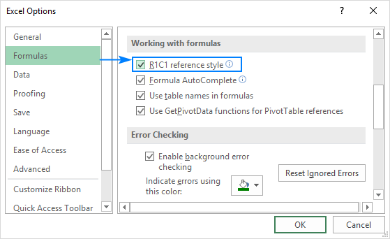
The below screenshot illustrates both the A1 and R1C1 reference styles:

To switch from the default A1 style to R1C1, click File > Options > Formulas, and then uncheck the R1C1 reference style box.
How to create a reference in Excel
To make a cell reference on the same sheet, this is what you need to do:
- Click the cell in which you want to enter the formula.
- Type the equal sign (=).
- Do one of the following:
- Type the reference directly in the cell or in the formula bar, or
- Click the cell you want to refer to.
- Type the rest of the formula and press the Enter key to complete it.
For example, to add up the values in cells A1 and A2, you type the equal sign, click A1, type the plus sign, click A2 and press Enter:

To create a range reference, select a range of cells on the worksheet.
For example, to add up the values in cells A1, A2 and A3, type the equal sign followed by the name of the SUM function and the opening parenthesis, select the cells from A1 through A3, type the closing parenthesis, and press Enter:

To refer to the whole row or entire column, click the row number or the column letter, respectively.
For instance, to add up all the cells in row 1, start typing the SUM function, and then click the header of the first row to include the row reference in your formula:

Tip. To get various information about a cell, use the CELL function.
How to change Excel cell reference in a formula
To change a cell address in an existing formula, carry out these steps:
- Click on the cell that contains the formula and press F2 to enter the Edit mode, or double-click the cell. This will highlight each cell/range referenced by the formula with a different color.
- To change a cell address, do any of the following:
- Select the reference in the formula and type a new one.
- Select the reference in the formula, and then select another cell or range on the sheet.

- To include more or fewer cells in a reference, drag the color-coded border of the cell or range.

- Press the Enter key.
How to cross reference in Excel
To refer to cells in another worksheet or a different Excel file, you must identify not only the target cell(s), but also the sheet and workbook where the cells are located. This can be done by using so-called external cell reference.
How to reference another sheet in Excel
To refer to a cell or a range of cells in another worksheet, type the name of the target worksheet followed by an exclamation point (!) before the cell or range address.
For example, here's how you can refer to cell A1 on Sheet2 in the same workbook:
=Sheet2!A1
If the name of the worksheet contains spaces or nonalphabetical characters, you must enclose the name within single quotation marks, e.g.:
='Target sheet'!A1
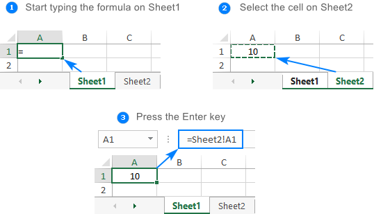
To prevent possible typos and mistakes, you can get Excel to create an external reference for you automatically. Here's how:
- Start typing a formula in a cell.
- Click the sheet tab you want to cross-reference and select the cell or range of cells.
- Finish typing your formula and press Enter.
For more information, please see How to reference cell in another worksheet in Excel.
How to reference another workbook in Excel
To refer to a cell or range of cells in a different Excel file, you need to include the workbook name in square brackets, followed by the sheet name, exclamation point, and the cell or a range address. For example:
=[Book1.xlsx]Sheet1!A1
If the file or sheet name contains non-alphabetical characters, be sure to enclose the path in single quotation marks, e.g.
='[Target file.xlsx]Sheet1'!A1
As with a reference to another sheet, you don't have to type the path manually. A faster way is to switch to the other workbook and select a cell or a range of cells there.
For the detailed guidance, please see How to reference cell in another workbook.
Relative, absolute and mixed cell references
There are three types of cell references in Excel: relative, absolute and mixed. When writing a formula for a single cell, you can go with any type. But if you intend to copy your formula to other cells, it is important that you use an appropriate address type because relative and absolute cell references behave differently when filled to other cells.
Relative cell reference in Excel
A relative reference is the one without the $ sign in the row and column coordinates, like A1 or A1:B10. By default, all cell addresses in Excel are relative.
When moved or copied across multiple cells, relative references change based on the relative position of rows and columns. So, if you want to repeat the same calculation across several columns or rows, you need to use relative cell references.
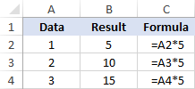
For example, to multiply numbers in column A by 5, you enter this formula in B2:
=A2*5
When copied from row 2 to row 3, the formula will change to:
=A3*5
For more information, please see Relative reference in Excel.
Absolute cell reference in Excel
An absolute reference is the one with the dollar sign ($) in the row or column coordinates, like $A$1 or $A$1:$B$10.
An absolute cell reference remains unchanged when filling other cells with the same formula. Absolute addresses are especially useful when you want to perform multiple calculations with a value in a specific cell or when you need to copy a formula to other cells without changing references.
For example, to multiply the numbers in column A by the number in B2, you input the following formula in row 2, and then copy the formula down the column by dragging the fill handle:
=A2*$B$2
The relative reference (A2) will change based on a relative position of a row where the formula is copied, while the absolute reference ($B$2) will always be locked on the same cell:

More details can be found in Absolute reference in Excel.
Mixed cell reference
A mixed reference contains one relative and one absolute coordinate, like $A1 or A$1.
There may be many situations when only one coordinate, column or row, should be fixed.
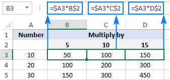
For example, to multiply a column of numbers (column A) by 3 different numbers (B2, C2 and D2), you put the following formula in B3, and then copy it down and to the right:
=$A3*B$2
In $A3, you lock the column coordinate because the formula should always multiply the original numbers in column A. The row coordinate is relative since it needs to change for other rows.
In B$2, you lock the row coordinate to tell Excel always to pick the multiplier in row 2. The column coordinate is relative because the multipliers are in 3 different columns and the formula should adjust accordingly.
As the result, all the calculations are performed with a single formula, which changes properly for each row and column where it is copied:
For real-life formula examples, please check out Mixed cell references in Excel.
How to switch between different reference types
To switch from a relative reference to absolute and vice versa, you can either type or delete the $ sign manually, or use the F4 shortcut:
- Double-click the cell that contains the formula.
- Select the reference you want to change.
- Press F4 to toggle between the four reference types.
Repeatedly hitting the F4 key switches the references in this order: A1 > $A$1 > A$1 > $A1.
Circular reference in Excel
In simple terms, a circular reference is the one that refers back to its own cell, directly or indirectly.
For example, if you put the below formula in cell A1, this would create a circular reference:
=A1+100
In most situations, circular references are a source of trouble and you should avoid using them whenever possible. In some rare case, however, they could be the only possible solution for a specific task.
The following tutorial explains how to find and remove circular references in Excel.
3D reference in Excel
3-D reference refers to the same cell or range of cells on multiple worksheets.
For example, to find an average of values in cells A1 to A10 in Sheet1, Sheet2 and Sheet3, you can use the AVERAGE function with a 3d reference:
=AVERAGE(Sheet1:Sheet3!A1:A3)
To make a formula with a 3d reference, here's what you need to do:
- Start typing a formula in a cell as usual, in this example we type =AVERAGE(
- Click the tab of the first sheet to be included in the 3d reference.
- Hold the Shift key and click the tab of the last sheet.
- Select the cell or range of cells to be calculated.
- Finish typing the formula and press the Enter key to complete it.
For more details, please see 3D reference in Excel.
Excel structured reference (table references)
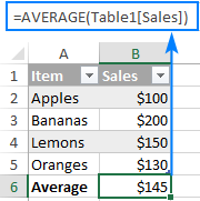
Structured reference is a special term for including table and column names in a formula instead of cells addresses. Such references can only be used for referring to cells in Excel tables.
For example, to find an average of numbers in the Sales column of Table1, you can use this formula:
=AVERAGE(Table1[Sales])
For more information, please see Structured refereces in Excel.
Excel names (named range)
An individual cell or a range of cells in Excel can also be defined by name. For this, you simply select a cell(s), type a name into the Name Box, and press the Enter key.
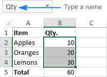
Upon creating new names, you may wish to replace the existing cell references in your formulas with the defined names. Here's how:
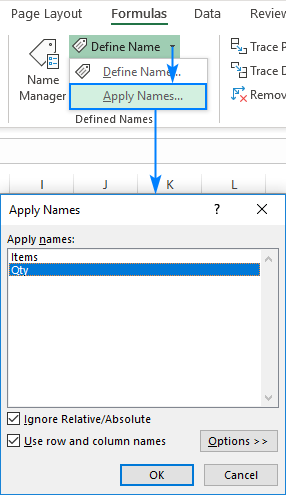
- Select the cells with the formulas in which you wish to change cell references to names.
To replace the references with defined names in all formulas on the active sheet, select any single blank cell.
- Go to the Formulas tab > Defined Names group, click the arrow next to Define Name, and then click Apply Names…
- In the Apply Names dialog box, select one or more names, and click OK.
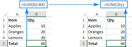
As the result, the references in all or selected formulas will be updated to the corresponding names:
The detailed information on Excel names can be found in How to create and use a named range in Excel.
That's how you work with cell references in Excel. I thank you for reading and hope to see you on our blog next week!
 by
by
88 comments
hmmmmm.........maybe it is possible for a 63-year-old guy to learn this after all!!
Hi! This is a fantastically comprehensive guide, which makes me wonder if what I'm looking for is possible.
My work uses a spreadsheet for weekly planning, but some rules work across 2 weeks, eg 1 & 2, 3 & 4 (but never 2 & 3). This means that I have a setup for odd weeks and even weeks, but it's a nuisance to have to manually edit the cross-sheet formulae every time I create a new pair. Is there a way, for example, to reference "one sheet to the left"? So instead of an absolute sheet name in the reference, something like sheet(currentSheet.index-1)![Cell reference] ?
Thanks!
Hi! You can create a dynamic reference to a sheet using a value in a cell. This can be done using the INDIRECT function and these instructions: Creating an Excel dynamic reference to another sheet.
I am trying to create a set of calculations where multiple make reference to the cell above them. I trying to use OFFSET(INDIRECT(CELL("address")),-1,0)/RP[[#Totals],[Unit]] where RP is a named range and Unit is a column header. For some reason it only works once on a sheet. If I try to use it in a second cell it changes the the first to the out come of the second. Doing some error checking I found that when i enter a new =Cell("address"), no matter where it is in the sheet, all the previous incidences will always return the same value as the newest instance. Is there a way around this so that each =Cell("address") returns the correct value for that particular cell?
Hello Sam!
The CELL function always returns the address of the current cell, i.e., the last cell that was modified manually.
It always refers to the current cell, no matter how many times it is used on the sheet.
Read more: Excel CELL function with formula examples.
If you need to get address of different cells, use other functions like =ADDRESS(row, column) or =CELL("address", reference), where reference is a reference to a specific cell.
Unfortunately I can't offer you a solution as I don't really understand what you want to do. Explain it in more detail and I will try to help you.
Thank you for your formula
Hello,
I manually update the Income Statement each month by inputting figures to each account within each organizations by month. I need a formula that can update the new figures to the corresponding cells in the Income statement by organization, then month and finally to the respective account.
This formula ='[TB JULY GOV TEST COPY.xlsx]Table 1'!Q4 works to updates figures. However, the formula is not able to distinguish between organization, month, or account.
Roughly, this is what my Income Statement looks like:
Cell A1: Org. 1.01
Cell A2:A100: Account Numbers
Cell B1: Account description
Cells B2:N2: Jan – Dec
I can provide screenshot if necessary. Appreciate any insight you can provide. Thank you!
Hi! Your data is not very clear to me. I can guess that you can use the SUMIFS function and this guide to calculate the sum of the conditions: Excel SUMIFS and SUMIF with multiple criteria – formula examples.
Hi,
With vlookup formula, I could able to pull a value from another sheet.
Now I want to know from address/number of that cell from where the vlookup has brought the value.
Eg: In a table, there are values in 4 columns (column A, B, C & D) in sheet1.
In sheet2, I put a vlookup formula (with several conditions) in cell C2 with the reference of table in sheet1 and I got the answer as 500.
Now, I want to know the cell address of this 500 value which is in the table of sheet1.
In sheet1, in all the 4 columns the value lies in column D but I want to know the cell address of this 500.
Sorry for my english.
Thank you
Hi! If I understand your task correctly, try the following formula:
=CELL("address",INDIRECT("D"&ROW(D2)-1+MATCH(VLOOKUP(F1,A2:D20,4,FALSE),D2:D20,0)))
Read more: Excel CELL function with formula examples.
Sub Copy_Example()
Range("B1").Copy Destination:=Worksheets("Sheet1").Range("C1:C(G1)")
End Sub
I want to change the desired range every time based on the number inside the G1 cell? example G1=10 then c1:C10 OR G1=20 Then C1:C20 And ...
Your request goes beyond the advice we provide on this blog. If you have a specific question about a function or formula, I will try to answer it.
Good evening, this helped me incredibly!
I have a question still, it might be in here but I haven't been able to find it. The increasing a row each day from Pete Allen was close but not quite it. Apologies if I have skimmed over it and feel free to ask for more info if required.
I have a sheet where there are several individual cells that refers to a cell range which increases each day. Each is in their own respective column but not the same row.
As an example:
For the total of column A, yesterday's formula was =SUM(A82:A124), today it's =SUM(A82:A125) and tomorrow it'll be =SUM(A82:A126) and so on. There's at least a dozen other columns following the same format but the total of B is a few rows down so I cannot put absolute values for the top of the cell range, select the entire row and drag it down to copy and delete the former row.
Up until now I go through all the individual cells changing the last cell address of the cell ranges, the idea is to make them each refer to a single cell off the side so I only have to change the row number and they all change their formula's
Thank you for your time and thank you again in advance!
Hi! To avoid manually changing the formula when you add data, use a dynamic range as described in this guide: How to create and use dynamic named range in Excel.
You can also convert your data to an Excel table and refer to the columns of that table in the formula.
Hi I want to calculate value in first cell using formula with some reference cells and then keep answer, go to next cell use same formula with same reference cells but change data on reference cells without it affecting the first answer. please help
Hi! If two formulas refer to the same cells, both formulas will change. You can replace the first formula with its value using Paste Special.
hi uh i wanted to know how do i cell reference: All the cells of column A from row 2 to the end
Thanks
Hi! Type in cell = sign. Click the mouse to the first cell A2, and then press CTRL+SHIFT+DOWN ARROW to expand the selection to the last cell in the column. Press ENTER.
Thank
How can i reference a cell and return the specific character count of 789.
A1: 12/99/904
Ref: A1 and Return 904 Which would be characters 7 and 8 and 9.
I am only looking for specific characters of that code but they are specifically characters 789. The number will change.
Hi!
To extract a certain number of characters from text, use the MID function.
If I understand your task correctly, try the following formula:
=MID(A1,7,3)
Thank you very much this is exactly what i was lookin for. I am very appreciative. I have learned a new tool for my excel tool box.
I have a master workbook to track employee paid time off - one worksheet for each employee. Separately, each employee has a workbook with one worksheet for each year they have worked. I want the worksheet in the employees workbook to auto-update from the master workbook I update each pay period. How do I link those for a dynamic connection? This would be an exact copy of the sheet from the master workbook.
Hi!
The following tutorial should help: Excel reference to another sheet or workbook (external reference).
My Question:
Step 1: I want to get the cell address in another cell (eg: I got cell address as "C2" in "F2")
Step 2: I want to add some value to that cell address to create new cell address (eg: I want to add 4 to "C2" which is available in "F2" and new cell address "C6" to be placed in "G2")
Step 3: I want to get the value of the cell address which I made in another cell (eg: the value of "C6" to be placed in "H2")
Hi!
To get cell address in cell F2, use CELL function: =CELL("address",C2)
To create a dynamic link, use the INDIRECT function. =INDIRECT(F2)
To create a link to a cell that is four rows lower than the original cell, use the OFFSET function =OFFSET(INDIRECT(F2),4,0)
I hope I answered your question.
How can I find a value (CTRL+F) in second sheet, if the second sheet has referenced values from master sheet or workbook? How can I search for a specific value in displayed values of References?
I need to change the formula to reference cell below, please advise
=VLOOKUP((B3-DAY(B3)+1),'2468 - North Trust'!$A$15:$G$48,6,FALSE)
i am working to return a value from the a second sheet to a master sheet. The second sheet values changes every 10 rows as there is a calculation with the second sheet. I have used the cell reference but this becomes tedious when i have close to a 1000 records and manually changing each takes along a time. Is there a way to resolve this programmatically?
Master sheet Call A1 = Second sheet A1
Master sheet Call A2 = Second sheet A10
Master sheet Call A3 = Second sheet A20
Hi!
To create a dynamic cell reference, use the INDIRECT function.
=INDIRECT("Sheet2!A"&(ROW(A2)*10))
Thanks for your insightful guides!
i am making one dataset using excel: column A stores the (univoque) ID for each data, then links between data are expressed in term of this ID.
Assume the following:
Links are stored in column L (so L = A#, since ID's are in A)
Properties (say a,b,c for simplicity) are stored in column P (P = "a" or "b" or "c")
i would like to do something like this
if (property(link) == "a", "Prop_A",property(link) == "b", "Prop_B",property(link) == "c", "Prop_C")
so basically i would like to check the property of the structure LINKED to the original one, and then provide an attribute based on this to the original structure)
how can this be done?
i hope i was clear enough sorry but i'm hardly wrapping my head around this
Hi!
Your explanations are not very clear. I assume that you will find this article useful to find the data you need: Excel INDEX MATCH - formula examples
If this does not help, explain the problem in detail.
This was exactly it!
i was looking for IF (INDEX (MATCH (...));then,else)
thank you so much
Sir, Match function returns me a row number(for example 66), how to use this row number in another match function to refer B66. how can i call 66 in match(A2,B[66],0)
Hi!
To create a cell reference from a text string, use INDIRECT function.
I can't get the relative row reference to change across columns when I am using an IF statement. (it works outside of the IF statement)
For example:
=IF([Book1.xlsx]Sheet1!$A1="P","P","") when I copy ACROSS the columns, the row number doesn't change. It only changes if I copy DOWN the columns.
Is there something I can do instead of manually typing in all row number changes for each cell across the columns?
Hello!
The $ sign means that when you copy the formula, the column address will not change. For more information see this guide: Relative and absolute cell reference: why use $ in Excel formula.
Hi,
I am trying to cross reference two spread sheets so I can see a list of people that is not on one that is on the other. I am not sure how to go about this. What would my formula be?
Thank you!!
Hello!
To compare two columns in tables, you can use these formulas and guidelines.
To find unique values in two tables, use the special Compare Sheets tool. It is available as a part of our Ultimate Suite for Excel which contains over 60 new features and improvements.