Comparing columns in Excel is something that we all do once in a while. Microsoft Excel offers a number of options to compare and match data, but most of them focus on searching in one column. In this tutorial, we will explore several techniques to compare two columns in Excel and find matches and differences between them.
How to compare 2 columns in Excel row-by-row
When you do data analysis in Excel, one of the most frequent tasks is comparing data in each individual row. This task can be done by using the IF function, as demonstrated in the following examples.
Example 1. Compare two columns for matches or differences in the same row
To compare two columns in Excel row-by-row, write a usual IF formula that compares the first two cells. Enter the formula in some other column in the same row, and then copy it down to other cells by dragging the fill handle (a small square in the bottom-right corner of the selected cell). As you do this, the cursor changes to the plus sign:
To find cells within the same row having the same content, A2 and B2 in this example, the formula is as follows: To find cells in the same row with different values, simply replace the equals sign with the non-equality sign (<>): And of course, nothing prevents you from finding both matches and differences with a single formula: Or The result may look similar to this:
As you see, the formula handles numbers, dates, times and text strings equally well. Tip. You can also compare two columns row-by-row using Excel Advanced Filter. Here is an example showing how to filter matches and differences between 2 columns.Formula for matches
=IF(A2=B2,"Match","")
Formula for differences
=IF(A2<>B2,"No match","")
Matches and differences
=IF(A2=B2,"Match","No match")
=IF(A2<>B2,"No match","Match")
Example 2. Compare two lists for case-sensitive matches in the same row
As you have probably noticed, the formulas from the previous example ignore case when comparing text values, as in row 10 in the screenshot above. If you want to find case-sensitive matches between 2 columns in each row, then use the EXACT function:
=IF(EXACT(A2, B2), "Match", "")
To find case-sensitive differences in the same row, enter the corresponding text ("Unique" in this example) in the 3rd argument of the IF function, e.g.:
=IF(EXACT(A2, B2), "Match", "Unique")
Compare multiple columns for matches in the same row
In your Excel worksheets, multiple columns can be compared based on the following criteria:
- Find rows with the same values in all columns (Example 1)
- Find rows with the same values in any 2 columns (Example 2)
Example 1. Find matches in all cells within the same row
If your table has three or more columns and you want to find rows that have the same values in all cells, an IF formula with an AND statement will work a treat:
=IF(AND(A2=B2, A2=C2), "Full match", "")
If your table has a lot of columns, a more elegant solution would be using the COUNTIF function:
=IF(COUNTIF($A2:$E2, $A2)=5, "Full match", "")
Where 5 is the number of columns you are comparing.
Example 2. Find matches in any two cells in the same row
If you are looking for a way to compare columns for any two or more cells with the same values within the same row, use an IF formula with an OR statement:
=IF(OR(A2=B2, B2=C2, A2=C2), "Match", "")
In case there are many columns to compare, your OR statement may grow too big in size. In this case, a better solution would be adding up several COUNTIF functions. The first COUNTIF counts how many columns have the same value as in the 1st column, the second COUNTIF counts how many of the remaining columns are equal to the 2nd column, and so on. If the count is 0, the formula returns "Unique", "Match" otherwise. For example:
=IF(COUNTIF(B2:D2,A2)+COUNTIF(C2:D2,B2)+(C2=D2)=0,"Unique","Match")
How to compare two columns in Excel for matches and differences
Suppose you have 2 lists of data in Excel, and you want to find all values (numbers, dates or text strings) which are in column A but not in column B.
For this, you can embed the COUNTIF($B:$B, $A2)=0 function in IF's logical test and check if it returns zero (no match is found) or any other number (at least 1 match is found).
For instance, the following IF/COUNTIF formula searches across the entire column B for the value in cell A2. If no match is found, the formula returns "No match in B", an empty string otherwise:
=IF(COUNTIF($B:$B, $A2)=0, "No match in B", "")
Tip. If your table has a fixed number of rows, you can specify a certain range (e.g. $B2:$B10) rather than the entire column ($B:$B) for the formula to work faster on large data sets.
The same result can be achieved by using an IF formula with the embedded ISERROR and MATCH functions:
=IF(ISERROR(MATCH($A2,$B$2:$B$10,0)),"No match in B","")
Or, by using the following array formula (remember to press Ctrl + Shift + Enter to enter it correctly):
=IF(SUM(--($B$2:$B$10=$A2))=0, " No match in B", "")
If you want a single formula to identify both matches (duplicates) and differences (unique values), put some text for matches in the empty double quotes ("") in any of the above formulas. For example:
=IF(COUNTIF($B:$B, $A2)=0, "No match in B", "Match in B")
How to compare two lists in Excel and pull matches
Sometimes you may need not only match two columns in two different tables, but also pull matching entries from the lookup table. Microsoft Excel provides a special function for this - the VLOOKUP function. As an alternative, you can use a more powerful and versatile INDEX MATCH formula. The users of Excel 2021 and Excel 365, can accomplish the task with the XLOOKUP function.
For example, the following formulas compare the product names in columns D against the names in column A and pull a corresponding sales figure from column B if a match is found, otherwise the #N/A error is returned.
=VLOOKUP(D2, $A$2:$B$6, 2, FALSE)
=INDEX($B$2:$B$6, MATCH($D2, $A$2:$A$6, 0))
=XLOOKUP(D2, $A$2:$A$6, $B$2:$B$6)
For more information, please see How to compare two columns using VLOOKUP.
If you don't feel very comfortable with formulas, you can have the job done using a fast and intuitive solution - Merge Tables Wizard.
Compare two lists and highlight matches and differences
When you compare columns in Excel, you may want to "visualize" the items that are present in one column but missing in the other. You can shade such cells in any color of your choosing by using the Excel Conditional Formatting feature and the following examples demonstrate the detailed steps.
Example 1. Highlight matches and differences in each row
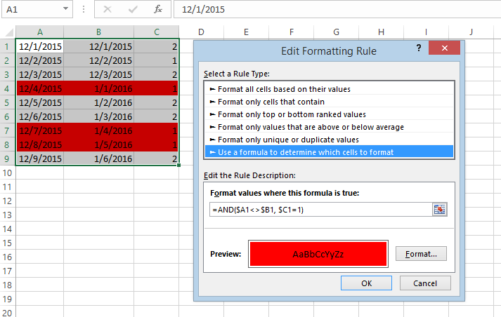
To compare two columns and Excel and highlight cells in column A that have identical entries in column B in the same row, do the following:
- Select the cells you want to highlight (you can select cells within one column or in several columns if you want to color entire rows).
- Click Conditional formatting > New Rule… > Use a formula to determine which cells to format.
- Create a rule with a simple formula like
=$B2=$A2
(assuming that row 2 is the first row with data, not including the column header). Please double check that you use a relative row reference (without the $ sign) like in the formula above.
To highlight differences between column A and B, create a rule with this formula:
=$B2<>$A2
If you are new to Excel conditional formatting, please see How to create a formula-based conditional formatting rule for step-by-step instructions.
Example 2. Highlight unique entries in each list
Whenever you are comparing two lists in Excel, there are 3 item types that you can highlight:
- Items that are only in the 1st list (unique)
- Items that are only in the 2nd list (unique)
- Items that are in both lists (duplicates) - demonstrated in the next example.
This example demonstrates how to color the items that are only in one list.
Supposing your List 1 is in column A (A2:A6) and List 2 in column C (C2:C5). You create the conditional formatting rules with the following formulas:
Highlight unique values in List 1 (column A):
=COUNTIF($C$2:$C$5, $A2)=0
Highlight unique values in List 2 (column C):
=COUNTIF($A$2:$A$6, $C2)=0
And get the following result:
Example 3. Highlight matches (duplicates) between 2 columns
If you closely followed the previous example, you won't have difficulties adjusting the COUNTIF formulas so that they find the matches rather than differences. All you have to do is to set the count greater than zero:
Highlight matches in List 1 (column A):
=COUNTIF($C$2:$C$5, $A2)>0
Highlight matches in List 2 (column C):
=COUNTIF($A$2:$A$6, $C2)>0
Highlight row differences and matches in multiple columns
When comparing values in several columns row-by-row, the quickest way to highlight matches is creating a conditional formatting rule, and the fastest way to shade differences is embracing the Go To Special feature, as demonstrated in the following examples.
Example 1. Compare multiple columns and highlight row matches
To highlight rows that have identical values in all columns, create a conditional formatting rule based on one of the following formulas:
=AND($A2=$B2, $A2=$C2)
or
=COUNTIF($A2:$C2, $A2)=3
Where A2, B2 and C2 are the top-most cells and 3 is the number of columns to compare.
Of course, neither AND nor COUNTIF formula is limited to comparing only 3 columns, you can use similar formulas to highlight rows with the same values in 4, 5, 6 or more columns.
Example 2. Compare multiple columns and highlight row differences
To quickly highlight cells with different values in each individual row, you can use Excel's Go To Special feature.
- Select the range of cells you want to compare. In this example, I've selected cells A2 to C8.
By default, the top-most cell of the selected range is the active cell, and the cells from the other selected columns in the same row will be compared to that cell. As you can see in the screenshot above, the active cell is white while all other cells of the selected range are highlighted. In this example, the active cell is A2, so the comparison column is column A.
To change the comparison column, use either the Tab key to navigate through selected cells from left to right, or the Enter key to move from top to bottom.
Tip. To select non-adjacent columns, select the first column, press and hold Ctrl, and then select the other columns. The active cell will be in the last column (or in the last block of adjacent columns). To change the comparison column, use the Tab or Enter key as described above.
- On the Home tab, go to Editing group, and click Find & Select > Go To Special… Then select Row differences and click the OK button.
- The cells whose values are different from the comparison cell in each row are colored. If you want to shade the highlighted cells in some color, simply click the Fill Color icon on the ribbon and select the color of your choosing.
How to compare two cells in Excel
In fact, comparing 2 cells is a particular case of comparing two columns in Excel row-by-row except that you don't have to copy the formulas down to other cells in the column.
For example, to compare cells A1 and C1, you can use the following formulas.
For matches:
=IF(A1=C1, "Match", "")
For differences:
=IF(A1<>C1, "Difference", "")
To learn a few other ways to compare cells in Excel, please see:
Formula-free way to compare two columns / lists in Excel
Now that you know Excel's offerings for comparing and matching columns, let me show you our own solution for this task. This tool is named Compare Two Tables and it is included in our Ultimate Suite.
The add-in can compare two tables or lists by any number of columns and both identify matches/differences (as we did with formulas) and highlight them (as we did with conditional formatting).
For the purpose of this article, we'll be comparing the following 2 lists to find common values that are present in both.
To compare two lists, here are the steps you need to follow:
- Start with clicking the Compare Tables button on the Ablebits Data tab.
- Select the first column/list and click Next. In terms of the add-in, this is your Table 1.
- Select the second column/list and click Next. In terms of the add-in, it is your Table 2, and it can reside in the same or different worksheet or even in another workbook.
- Choose what kind of data to look for:
- Duplicate values (matches) - the items that exist in both lists.
- Unique values (differences) - the items that are present in list 1, but not in list 2.
Since our aim is to find matches, we select the first option and click Next.
- This is the key step where you select the columns for comparison. In our case, the choice is obvious as we are only comparing 2 columns: 2000 Winners against 2021 Winners. In bigger tables, you can select several column pairs to compare by.
- In the final step, you choose how to deal with the found items and click Finish.
A few different options are available here. For our purposes, these two are most useful:
- Highlight with color - shades matches or differences in the selected color (like Excel conditional formatting does).
- Identify in the Status column - inserts the Status column with the "Duplicate" or "Unique" labels (like IF formulas do).
For this example, I've decided to highlight duplicates in the following color:
And in a moment, got the following result:
With the Status column, the result would look as follows:
Tip. If the lists you are comparing are in different worksheets or workbooks, it might be helpful to view Excel sheets side by side.
This is how you compare columns in Excel for matches (duplicates) and differences (unique values). If you are interested to try this tool, you are welcome to download an evaluation version using the below link.
I thank you for reading and encourage you to check out other helpful tutorials that we have :)
Available downloads
Compare Excel Lists - examples (.xlsx file)
Ultimate Suite - trial version (.exe file)
550 comments
Is there a way to compare data in one column to data in another column for mismatches and then have only the data that is different be highlighted or change the text color?
For example:
Col A Col B
State Farm State Frm In this example the "a" in Col A would be highlighted or a different color text
Hi! You can only compare the characters in two cells and highlight the color using a VBA macro.
Hello, would you mind sharing a VBA macro for this?
(only parts of the text in the cell that are different between 2 columns)
That'd very much helpful and appreciated!
Thank you so much!
Sorry, your request goes beyond the advice we provide on this blog.
Would you mind sharing the VBA macro for this? It will help a lot! Thank you so so much!
Hi, hoping you can answer an issue I am having. So eg. I have account numbers in column A, column B holds the users to that account number (there can be multiple users for one account) I need to pull the users of that one account into one cell…I then need to compare those results to column C (which holds the primary account user) and if it doesn’t match then return the value (user names). Is this achievable…?
Hi! Use the FILTER function to get an array of users with the account number that is written in D1. Then combine this into a delimited text string using the TEXTJOIN function.
Try this formula:
=TEXTJOIN(",",TRUE,FILTER(B2:B30,A2:A30=D1))
Selamat siang, saya memiliki 2 cell yang hampir mirip
Cell Sumber
A1 : Mei Jakarta 18
A2 : Mei Jakarta
Cell Hasil
A3 : 18
Apakah ada cara untuk memunculkan karakter yang tidak terduplikat di 2 atau lebih cell seperti contoh diatas?
terima kasih banyak
Hi! Combine the values into a text string with the TEXTJOIN function. Split this text string into separate words with the TEXTSPLIT function. Find unique words with the UNIQUE function.
=UNIQUE(TEXTSPLIT(TEXTJOIN(" ",TRUE,A1:A2),," "),FALSE,TRUE)
Hello,
If I have a large set of data and in each column is numbers for that specific value that makes it unique how can I compare that value to any other value like it and have them match up?
For example,
Peaches = 23, 44, 45, 67, 69, 50, 18, 16
Apples= 99, 44, 42, 67, 69, 40, 18, 16
and because they have 5 values in common I would want them to be highlighted or paired together some how.
Is this possible?
Thank you in advance
Correction** exact matches only.
Thank you
Hi! Maybe this article will be helpful: How to highlight duplicate cells and rows in Excel.
Hi,
I would like to compare and highlight same text string from 2 column.
Example:
D2 SALTED DUCK EGGS
F2 EGGS 360'S/CTN
I want compare these two column, search and highlight same text, EGGS
I have many rows need compare, D2 compare F2, D3 compare F3.
How to set formula, please advise, thanks~.
Hi! If you are looking for a specific word in the text, you can use these instructions: How to find substring in Excel.
If you are looking for any matching words, try Fuzzy Duplicate Finder. It is available as a part of our Ultimate Suite for Excel that you can install in a trial mode and check how it works for free.
I hope it’ll be helpful.
How I can compare only part of the text in two columns in the same row for this case:
Column A contains abc-123
Column B contains abc
I want column C to get FALSE if left part of the text in column A isn't the same.
Thank you!
Hi! We have a special tutorial on this. Please see: How to find substring in Excel
Try this formula:
=ISNUMBER(SEARCH(B1,A1))
Thank you so much!
I'd been looking for a formula forever, trying to figure out how to compare two columns of data (not just the corresponding rows) & have a separate column display whether one of the entries was unique to one list or not.
Many thanks :)
Hi
Could you please help me on below query.
In column a i have date and in column b i have date and other text.
How can I verify column a date and column b dates. If both are same
Hi!
If I understand correctly, you need to find a partial match of cell values. Use the TEXT function to convert the date to text in the correct format. Here is an example formula:
=ISNUMBER(SEARCH(TEXT(A1,"dd-mm-yy"),B1))
For more information, please read: How to find substring in Excel
how do we find true/false when cell "A" contain the name "a b c" and cell "B" contains the name "c a b"
Hi!
Your question is not very clear. To find a partial match of text strings, please read: How to find substring in Excel
Hi,
Is there a way to only highlight one set of duplicate in both columns?
If column A has the following numbers: 20, 21, 22, 23, 24 & 25
Then column B has the following numbers: 20, 20, 21, 22, 23, 20 & 25
Could only (1) of the 20s in column B be highlighted leaving the other 20 un-highlighted?
Hi!
If I understand the problem correctly, add another condition to the conditional formatting formula:
=AND(COUNTIF($C$2:$C$20, $A2)>0, COUNTIF($A$2:$A2, $A2)=1)
The second condition will allow only the first duplicate in the column to be highlighted with color.
Hello Alexander,
I believe you are close to figuring out my issue. If I use my example above, from A2-A7 I have entered 20, 21, 22, 23, 24 & 25 and from C2-C8 I have entered 20, 20, 21 22, 23, 20 & 25. After entering your formula, the first set of 20s are highlighted in cells A2 & C2 while the 20s in C3 & C7 are not highlighted - this is what I was looking for, thank you! However, the 21 in cell A3 is not highlighted while the 21 in cell C4 is highlighted. Additionally, the 24 in cell A6 is highlighted when there is not a duplicate 24 in column C.
I am looking to review a large set of numbers in (2) columns to see if the costs from one column are reflected in the 2nd. If the costs are only in (1) column then I will know something needs to happen in my budget to bring it back to normal. However, there will likely be the same number multiple times in both columns and I need a way to show which did not get reflected in the 2nd column. Please let me know if this situation makes sense or if there is a way to share my worksheet.
Thank you,
Gary
Hi!
I used your data and the conditional formatting formula suggested above for column A. Cells A2,A3,A4,A5 were highlighted. A6 - not highlighted.
I don't know what conditional formatting formula you used for column C.
In first cell I have values like A,B,C and in 2nd cell I have value of B,A,C in this case both cell values are same but sequence is not match I want return value as True and if any value missed then false how to do it in excel
Hi!
Excel cannot compare text strings with different word orders. Split each text string into cells using a comma as a separator. You can read more about this here: Split string by delimiter or pattern, separate text and numbers or TEXTSPLIT function in Excel: split text strings by delimiter. Then compare the values using the IF function with AND and OR statements.
Thank you very much Alexander Trifuntov. Was looking for this for almost 4 hours.
Thank you once again for sharing the Template.
God Bless.
Thank you for your explanation but is there a function to know if two cells are on the same row in an other sheet ?
Hello!
I am not sure I fully understand what you mean. You can get the row number using the ROW function or CELL function
Good evening,
I have a unique 'multi-condition' question I'm using for scaled criteria in Excel.
I am matching paygrades (determined by O2, O3, O4, etc)
--but I am scaling their qualitative value based on if their paygrade matches the paygrade requirement of the job.
I am scaling it where:
If the paygrades match, they get a 5 (highest),
If they don't match (and only differ by one paygrade), they get a 3 (medium).
If the paygrades don't match, but differ by More than 1, they get a 1 (lowest).
End state: trying to maximize matching ability with scaled scores, but I'm struggling to do a multi-IF function
--without needing to manually change the 3's (non-match) for those who differ by more than 1 paygrade to a 1.
I hope that makes sense.
In a large file, I require a formula that can do this.
Thank you in advance for any assistance on the formula I need to input (after hours of searching for the code).
Sincerely,
--Josh
Hi!
Your task is not completely clear to me. To understand what you want to do, give an example of the source data and the desired result.
Good day sir,
Pardon the confusion, but please see below for reference:
Data: Military Officers Matched to the Billet (Job) they fill, based on their paygrades (indicates their experience)
Two columns:
Column A is the Person's paygrade
Column B is the Billet (Job's) required paygrade
I wish to assign values, 1, 3 or 5, based on how Personnel paygrade match (or differ) from the Billet (job) paygrade requirement
IE:
If an O6 is filling an O6 job, value = 5
If an O6 is filling an O5 job, value = 3
If an O6 is filling an O4 job, value = 1
Bottom line:
if the Person paygrade (column A) matches requirement (column B) = 5
If the person paygrade does NOT match requirement (differs by just 1) = 3
If the person paygrade does NOT match requirement (differs by >1) = 1
These values go into a (200x200) Matrix of all possible combinations (Personnel paygrade to Job paygrade requirement),
--which will then be 'scaled' against monetized benefits of their 'possible' combinations
Then this will be compared to a similar Matrix of monetized costs
I hope this makes more sense.
I just need a formula that can be dragged across various rows/columns to find these values (5, 3, 1)
Thank you for any assistance.
Sincerely,
--Josh
Hello!
The information you provided is not enough to understand your case and give you any advice, sorry.
Give me some data examples for the cells you mentioned and the desired results.
Thanks for your excellent advice! I have a slightly more complicated "duplicated cells" comparison that I cannot solve. I have 2 columns of several hundred mosquito trap locations each (the cells contain addresses primarily, but some free text). I need to determine which cells are duplicates. However, the spelling could be slightly different in each column. For example, a cell in Column A has "1st Presbyterian Church" and a cell in Column B has "1st Pres Church". Another in Column A has "2208 GRANDHAVEN DR CONCORD NC 28027" and Column B has "2208 GRANDHAVEN DR". In both cases, these are the same location in reality, but because the text is not exact, do not result out as duplicates in the COUNTIF functions I have attempted. Is it possible to write a function for partial matches... such as matches for "2208" or "Pres" that would highlight the all cells that contain matching strings of numbers or text?. Thanks for any advice offered.
Hi!
You can identify cells with partial text matches using the Duplicate Remover - Fuzzy Duplicates Finder tool. It is available as a part of our Ultimate Suite for Excel that you can install in a trial mode and check how it works for free.
Hello, I need to compare 2 columns, one is the status of something (complete, not complete, in process, stalled), and the other would be how many items have been ordered ONLY IF the status is "complete", but I am failing at every equation I try, help?
Hi!
The information you provided is not enough to understand your case and give you advice. I don't know how you want to compare columns. For example, instead of using the COUNTIF function, you can use COUNTIFS to take into account the status.
Please clarify your specific problem or provide additional information to understand what you need.
Column1 Column2
Andy JOHNSON Andrew Johnson
How can I highlight the difference in letters in this two names with another color ?
Hi!
In Excel, you can only conditionally format an entire cell, not individual characters.
Hi,
Thank for the great article.
Every singel one of this formulas gives me an "There is a problem with this formula" error when copy/pasting them into Excel...what am I doing wrong?
Sorry, just found out. Your commas are semicolons on my Excel, no clue why, but took me a while to find out ;)
I have to compare four column in two sheets. Like
Sheet 1:
column G "DHKMTRTA138217, DHKMTRTA162534,......... and Column E "DHAKA METRO-TA-13-8217", "DHAKA METRO-16-2534",...........
Sheet 2:
Column A "DHKMTRTA138217", "DHKMTRTA162534",.........
I need a result in Column C of Sheet 2 "DHAKA METRO-TA-13-8217", "DHAKA METRO TA-16-2534",....... (Result need to pick from Sheet 1 column E)
Would you kind help me to get the result
Thank you
Jewel
Hi!
You can select the result with the VLOOKUP or INDEX+MATCH function.
I want that the values in Column B to Column Z gets highlighted as per the values entered in Column A. Two conditions for getting highlighted are 1.) When it is equal to or greater than the value of Column A
2.) When it is in between the range of 90% to 99.99% of the value of Column A.
Hi!
For each column from B to Z, create a conditional formatting rule. I recommend reading this guide: Excel Conditional Formatting tutorial with examples. Use the Highlight Cell Rules option or conditional formatting formula, ex. =A1 < B1