This tutorial explains the most common mistakes when making formulas in Excel, and how to fix a formula that is not calculating or not updating automatically.
Can someone imagine using Microsoft Excel without formulas? I believe no one can. And hardly anything could compare to the frustration caused by Excel formulas stop working all of a sudden. When this happens, a bunch of questions immediately flash across your mind. Why is my Excel formula not calculating? Why doesn't this formula update its value automatically? Is my Excel corrupt or is this due to some malicious virus? And how do I get my Excel to calculate and update formulas automatically again? Don't worry, most likely your Excel is all right, and you will get all the answers in a moment.
Excel formulas not working
Symptoms: Excel formula not working correctly, it returns an error or a wrong result.
This section provides a summary of the most common mistakes people make when creating formulas in Excel and solutions to fix them.
1. Match all opening and closing parentheses in a formula
As you know, the arguments of Excel functions are entered within the parentheses. In complex formulas, you may need to enter more than one set of parentheses, one within another, to indicate the order in which the calculations should take place. When creating such a formula, be sure to pair the parentheses properly so that you always have a right parenthesis for every left parenthesis in your formula.
Microsoft Excel displays the parentheses pairs in different colors as you enter them in a formula. If your formula is short of one or more parentheses, Excel displays an error message and suggests a correction to balance the pairs. Please see How to highlight and match parenthesis pairs for more information.
2. Enter all required arguments in an Excel function
All Excel functions have one or more required arguments. Some functions also have optional arguments, which are enclosed in [square brackets] in the formula's syntax.
A formula must contain all of the required arguments, otherwise Excel displays "You've entered too few arguments for this function" alert.
If you have entered more arguments than allowed by the formula's syntax, you will get "You've entered too many arguments for this function" error message.
3. Do not nest more than 64 functions in a formula
When nesting two or more Excel functions into each other, e.g. creating a nested IF formula, remember about the following limitations:
- In Excel 2016, Excel 2013, Excel 2010 and Excel 2007, you can use up to 64 nested functions.
- In Excel 2003 and lower, only up to 7 nested functions can be used.
4. Don't enclose numbers in double quotes
In Excel formulas, any value enclosed in double quotes is interpreted as a text string.
What it means is that if you enter a formula like =IF(A1>0, "1"), Excel will treat number 1 as text, and therefore you won't be able to use the returned 1's in other calculations. To fix this, just remove the double quotes around "1": =IF(A1>0, 1).
So, whenever you are writing a formula for numerical values, follow this simple rule: don't enclose numbers in double quotes unless you want them to be treated as text.
5. Enter numbers without any formatting
When using a number in an Excel formula, don't add any decimal separator or currency sign like $ or €.
Remember that in Excel formulas, a comma is typically used to separate a function's arguments, and the dollar sign makes an absolute cell reference.
For instance, instead of entering $50,000 in your formula, input simply 50000, and use the Format Cells dialog (Ctrl + 1) to format the output to your liking.
6. Make sure numbers are not formatted as text values
Numbers formatted as text values are another common reason for Excel formulas not working. At first sight, they look like normal numbers, but Microsoft Excel perceives them as text strings and leaves out of calculations.
The visual indicators of text-numbers are as follows:
- Numbers formatted as text are left-aligned by default, while normal numbers are right-aligned in cells.
- The Number Format box on the Home tab in the Number group displays the Text format.
- When several cells with text numbers are selected on the sheet, the Status Bar only shows Count, while usually it shows Average, Count and SUM for numbers.
- There may be a leading apostrophe visible in the formula bar, or green triangles appear in the top-left corner of the cells.
The below screenshot shows that even a simple Excel SUM formula may not work because of numbers formatted as text:

To fix this, select all problematic cells, click the warning sign, and then click Convert to Number:
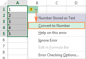
In some cases, however, neither green triangles nor the warning sign appear in cells. For example, if you enclose numeric values in double quotes in your formulas, Excel assumes you want to output a text string rather than a number.
At first sight, the following formula appears to be working fine:
=IF(A1="Good", "1", "0")
But the problem is the returned 1's and 0's are text values, not numbers! And if you reference any cells with the above formula in other formulas, those cells won't be included in calculations. As soon as you remove "" surrounding 1 and 0 in the above formula, Excel will treat the outputs as numbers and they will be calculated correctly.
If the small green triangles do not appear in cells for some other reason, look at the Number Format box on the Home tab in the Number group. If it displays Text, try clearing all formatting for the problematic cells, and set the cells' format to Number or General. If that doesn't work, you might have to create a new column, manually input the data (e.g. copy your text-numbers to Notepad, and then back to a new column), and delete the broken column.
Another possible solution is to multiply the values in the problematic column by 1 using a simple formula like =A1*1. And then, copy the formula cells and paste them as values in the same or in any other column via Paste Special > Values.
7. Separate function arguments with a proper character
Most of us are used to separating function arguments with commas. However, this does not work for everyone's Excel. The character you use to separate arguments depends on the List Separator set in your Regional Settings.
Comma is the default list separator in North America and some other countries. In European countries, comma is used as the decimal symbol and the list separator is usually set to semicolon.
For example, in North America you would write =IF(A1>0, "OK", "Not OK"), while European users of Excel should put the same formula as =IF(A1>0; "OK"; "Not OK").
So, if your Excel formulas are not working because of "We found a problem with this formula..." error, go to your Regional Settings (Control Panel > Region and Language > Additional Settings) and check what character is set as List Separator there. And then, use exactly that character to separate arguments in your Excel formulas.
8. Enclose workbook and worksheet names in single quotes
When referring to other worksheets or workbooks that have spaces or non-alphabetical characters in their names, enclose the names in 'single quotation marks'. For example,
Reference to another sheet:
=SUM('Jan Sales'!B2:B10)
Reference to another workbook:
=SUM('[2015 Sales.xlsx]Jan sales'!B2:B10)
For more information, please see How to refer to another sheet or workbook in Excel.
9. Include the full path to a closed workbook
If you are writing a formula that references a closed Excel workbook, your external reference must include the workbook name and entire path to the workbook. For example:
=SUM('D:\Reports\[Sales.xlsx]Jan'!B2:B10)
For more information, please see Creating a reference to another workbook.
If the above tips do not help, try to evaluate and debug each part of your formula individually by using the F9 key and other debugging techniques explained in the following tutorial: How to evaluate and debug formulas in Excel.
Excel formulas not updating
Symptoms: The value returned by your Excel formula does not update automatically, i.e. the formula continues to show the old value even after you've changed the values of the dependent cells.
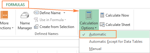
When Excel formulas are not updating automatically, most likely it's because the Calculation setting has been changed to Manual instead of Automatic. To fix this, just set the Calculation option to Automatic again.
On the Excel ribbon, go to the Formulas tab > Calculation group, click the Calculation Options button, and select Automatic:
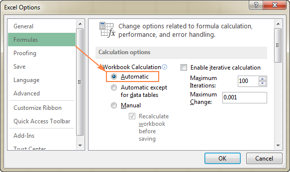
Alternatively, you can change this setting in Excel Options:
- In Excel 2003, click Tools > Options > Calculation > Calculation > Automatic.
- In Excel 2007, click Office button > Excel options > Formulas > Workbook Calculation > Automatic.
- In Excel 2010, Excel 2013, and Excel 2016, go to File > Options > Formulas > Calculation options section, and select Automatic under Workbook Calculation.
How to force Excel formulas to recalculate
If for some reason, you need to have the Calculation option set to Manual, you can force the formulas to recalculate by clicking the Calculate button on the ribbon or by using one of the following shortcuts:
To recalculate the entire workbook:
- Press F9, or
- Click the Calculate Now button on the Formulas tab > Calculation group.
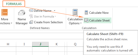
To recalculate an active sheet:
- Press Shift + F9, or
- Click Calculate Sheet on the Formulas tab > Calculation group.
To recalculate all sheets in all open workbooks, press Ctrl + Alt + F9.
If you need to recalculate only one formula on a sheet, select the formula cell, enter the editing mode either by pressing F2 or double clicking the cell, and then press the Enter key.
Excel formulas not calculating
Symptoms: A cell displays the formula, not the result.
If your Excel formula is not working because a cell displays the function instead of the calculated value, it's because one of the following reasons.
1. Show Formulas mode is turned on
The most common reason for an Excel formula not calculating is that you have inadvertently activated the Show Formulas mode in a worksheet.
To get the formula to display the calculated result, just turn off the Show Formulas mode by doing one of the following:
- Pressing the Ctrl + ` shortcut, or
- Clicking the Show Formulas button on the Formulas tab > Formula Auditing group.

2. A formula is entered as text
Another frequent reason for your Excel formula not calculating is that the formula has been formatted as text. To check this, select the formula cell, and look at the Number Format box in the Number group on the Home tab:
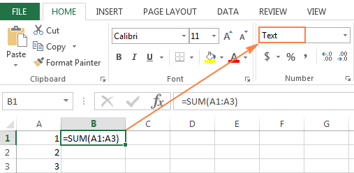
If it is the case, change the cell format to General, and while in the cell press F2 and Enter for the formula to recalculate and display the calculated value.
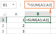
3. A formula cell has a leading space or apostrophe before the equal sign
If you have inadvertently entered a space or apostrophe (') before the equal sign, Excel treats the cell contents as text, and consequently does not evaluate any formula within that cell (a leading space often appears when you copy a formula from the web). To fix this, just remove the leading space or single quote.
This is how you deal with formulas not working in Excel. If you know any other solutions to fix formulas not updating or not calculating, please do share in comments. I thank you for reading and hope to see you on our blog next week.
 by
by
459 comments
I am using Microsoft® Excel® 2019 MSO (Version 2410 Build 16.0.18129.20158) 64-bit. Not finding unique and filter command. How to enable these commands in my version. Thanks
Hi! Currently, only Excel for Microsoft 365 and Excel 2021 have the UNIQUE function and FILTER function.
Check box do not show True or False in formula bar.
I am developing tracker for which I want to know the sum of all ticked columns by using countif command. System is returning 0. Not sure whether check box is activated or not automatically. How to get the count of ticks ???
Thanks b/regds,
Hi! You need to associate the checkbox with a specific cell to capture the checkbox state (checked or unchecked). Read more: How to link a checkbox to a cell. After that, you will be able to count the number of activated checkboxes with approximately this COUNTIF formula:
=COUNTIF(A1:A10,TRUE)
Hi, I can't get the total of time calculated on a specific column. Sum function doesnt work and sumifs doesnt work as well.
I would like to calculate how much time (hh:mm) is one person coming in late based off on a formulated result =TEXT(C2-$E$1,"hh:mm") -- this formula is based on an entered time (log-in), minus the expected time of log in. (to get the minutes of tardiness). For some reason I cannot use sumif to calculate how many minutes a specific staff is late for a period of time.
Thank you!!
Hi! TEXT function will return a string of text that you will not be able to do any calculation with. There is not enough information in your question to offer you another solution.
Maybe this article will help: Calculate time in Excel: time difference, add, subtract and sum times.
its not updating, i have to double click each cell and press enter for it to update
Hi! Pay attention to the following paragraph of the article above: Excel formulas not updating.
Hi, I created a formula in excel but now it refuses to add the column. No matter what I do to change the cell to a Number, General it refuses to acknowledge it as a number so I cannot auto sum the column.
=IF(BE8="AE",IFERROR(VLOOKUP(B8,'Paychex 2nd Bi-Weekly'!$I$5:$BU$197,15,0),0),"0")&IF(BE8="AE",IFERROR(VLOOKUP(B8,'Paychex 2nd Bi-Weekly'!$I$5:$BU$197,12,0),0),"0")
Hello Sondra!
Your IF formula always returns text, not a number. In the [value_if_true] argument, you combine two values using concatenation operator (&) and get text. In the [value_if_false] argument, you return the text string “0”. Therefore, you cannot do any calculations.
Maybe this guide will be helpful: Convert text to number.
Hi, my cell is linked to another cell to produce its value but it will only keep updating as 0. (cell i162 is a sum formula cell giving me a value. I am formulating cell j160= I162 but it is not showing the same value but rather a 0 and will not change) How can i fix this?
Hi! The formula j160= I162 can only return TRUE or FALSE (1 or 0), not the cell value. To assign a value to a cell, use a cell reference. Read more here: Excel cell reference: how to make and use.
Sorry the formula is not J160=I162, the Cell J160's value inputed '=I162' but will not have the updated value that is in I162
Hi! I can't see your worksheet, but I think that if you carefully study the recommendations in the article above, you will be able to solve the problem.
learned so much from this, ty!
these solutions did not fix my problem, but through reading, i got ideas that did. the short of it, i had some cells that were the result of a formala within a column where my column sum was no longer current, so i deleted the formulas for those cells, just wrote in their value, and then my column sum was correct.
love you a million for this help
I've come across an odd thing. Granted, this file is quite an entanglement and bogs down frequently, but this is the first I've seen of this.
I have a table that is used as a database to vlookup from another table/tab. I have a concatenate in both tables, first column, that pits an item number and store number together (columns B & F).
I've entered the simple formula "=CONCATENTATE(B2,F2)" and it is carried on down each row.
In the first table that is pulling data from this second table, the concatenate is working fine. But in this one, each cell in that column is a 0.
I've confirmed the formula is pulling the cells in correctly (vs 'B2' being text) by the way cells B2 & F2 are highlighted in color to match the text in the formula itself.
I've used 'Calculate Now', 'Calculate Sheet' and made sure 'Show Formulas' is switched correctly.
I've closed and reopened the file, as well as open an earlier version (saved as a different file from week prior) and it is working fine in that one.
I'm baffled.
I have a screenshot of the file that shows the anomaly, if needed.
Disregard.
I filtered column B and the formula kicked in. Unfiltered and all is good. Laptop or file just wanted to be a diva.
Hi - i have a complicted If/isnumber/search formula that is working beautifully ! as i drag it down a very long list of data that i am testing, it's working great! then suddenly not returing a result (other than "false" b/c it can't find what I'm testing for.
The thing is that the row immediately above it has the EXACT same info to be tested, and it returned a result, but the next row, didn't. and no subsequent row did - so my list is 35000 rows, and the formula just stopped returning ANYTHING on row 31825 for the rest of the list
Example: (testing for the word "car")
modern car - yes
modern car - FALSE
all formatting is exactly the same in each row & column
why would this happen?
Hi! Unfortunately, this information is not enough to give you advice. Without seeing your formula, I can't say anything about how it works or why it doesn't work. Also check if your text cells contain extra spaces or unprintable characters.
Try to follow the recommendations from this article: How to delete special / unwanted characters in Excel.
Thank you, but the real issue is why a formula would behave differently. I am well versed in Excel. All formatting and the data is EXACTLY the same in the next row and it still doesn't return a result. then, it just bascially stops returning results from there down.
Same spreadsheet I use daily just stopped adding totals correctly. When dragging cell data over, it drags the number, not the formula, even though the formula is showing. I tried to copy and paste formula but same thing is happening.
Have tried Calculate now and Calculate sheet but no change
Its a really simple calc just a A1+B1-C1. A1+B2 works, but when I add inC1 it just zeros out. Autosum also not working
Both B1 and C1 are total sums of other cells in the same row. It doesn't seem to be a circular reference issue.
I have tried every online check/fix I could find -
Enabled fill handle to drag is on
Formulas calculations are set to auto not manual
Data is set to number not text and there are no $ symbols,
I have run updates and rebooted my machine and tried copying line items and creating a new book but the same thing is happening.
I can't find any more online fixes that might relate, can you help?
thanks so much!
p.s Every other spreadsheet works fine!
Hi! Unfortunately, I have not been able to reproduce your problem. Check for circular references in all cells that have a link to cell C1.
thanks
I have the formula "=COUNT(IF(ISNUMBER(D13:K13),D13:K13))". It shows the value 1 no matter how many of the cells in the specified range are numbers. I have both the formula and the cells containing the numbers in number format. Same formula works in other excel files. I appreciate any comments.
Hi! I have this formula calculating the numbers correctly. Check, maybe your numbers are written as text. Read more: How to identify numbers formatted as text.
I've copied a sheet into Excel online and the formula I am using: =DATEDIF(C9, D9, "Y") is working for some cells in the column but not all. It works in the first 7 cells but not the next 4 and so on and I can't see anything wrong, I've tried all the usual things!
Hi! I can't check your formula because I don't have your data. What data is written in these cells? What error does the formula return? Check, it may be text written as a date. Maybe this article will be helpful: Excel DATEDIF to calculate date difference in days, weeks, months or years.
Hi Alexander. Thank you for replying. I have checked the cells and they are all set the same, as date in the UK format. This is the same with the cells that are returning the correct data and also the ones that are then simply showing #VALUE!
So all cells are formatted the exact same way but, once transferred into an Excel online sheet, it will only work on some, but not all cells in the same column.
C9 has the date in the same format as D9 for e.g. and the exact same formula works on several cells in a column then skips a few then works again. In the desktop version it works throughout the whole column with no errors at all.
I can't see how to post a screenshot or would do so.
Hi! If your date is written as text, it doesn't matter what format is set in the cell. I recommend reading this guide: How to distinguish normal Excel dates from "text dates". Also check that the default date formats are the same in desktop and online versions. If they are not the same, some dates may be converted to text when copied.
Hello,
Sometimes my formulas show as formula and sometimes as values. I cannot find the reason for this and I cannot get it working. I looked at the options of the calculations, data validation, regional settings, formula placed as 'general' not as text, removing possible spaces before the formula and still it does not work. Could you please help?
I am currently having troubles with this formula: =MID(RC[-3] SEARCH("(", RC[-3]) + 1, SEARCH(")", RC[-3]) - SEARCH("(", RC[-3]) - 1)
This formula was created as :
=MID(M2,SEARCH("(",M2)+1,SEARCH(")", M2) - SEARCH("(", M2) - 1)
But my excel cells showed RC[-3] when selecting text in column M2.
Hi! Unfortunately I cannot reproduce your problem. Have a look Formulas tab – Formula Auditing group – Show Formulas button. Also, if the cell is set to TEXT format, you may often see a formula instead of a value in Excel.
Thank you. Excellent tutorial. Step 2 solved my issue - I had inadvertently changed the formula to text.
Now my formulas are working again! thanks a lot for your information. Better than a chat IA bot ;)
Thank you for the article. It really helped troubleshoot the issue.
So I have this formula =IF(O69="Cup",L69*'Liquid Cost Sheet'!M116,IF(O69="Tbls",L69*'Liquid Cost Sheet'!Q116,IF(O69="Tsp",L69*'Liquid Cost Sheet'!U116,"0")))
I have used this on 50 different sheets and have now created a new sheet where the word "Cup" is not being recognized. I changed it to "Cups" and it works.
Hi! I can't check your formula because I don't have your data. There may be extra spaces or other characters in your data. Maybe this article will be helpful: How to compare two cells in Excel (string comparison).
The following table details the revenue by bank account number
Calculate the total revenue from "Gold" accounts in the State of NY
Account # Type State Revenue
1 Gold NY 492
2 Silver PA 124
3 Gold NJ 555
4 Gold NY 100
5 Bronze NY 8
6 Bronze MA 201
7 Gold NY 20
8 Silver PA 43
9 Gold PA 108
10 Bronze NJ 172
Answer: =SUMIFS(B4:B13,"Gold",C4:C13) Try again
Hi! I’m sorry, but your description doesn’t give me a complete understanding of your task. Correct me if I’m wrong, but I believe the formula below will help:
=SUMIFS(B4:B13,"Gold NY",C4:C13
Read more: Excel SUMIFS and SUMIF with multiple criteria – formula examples.