In this tutorial, we will be looking at how to use IFERROR and VLOOKUP functions together to trap and handle different errors. In addition, you are going to learn how to do sequential vlookups in Excel by nesting multiple IFERROR functions one onto another.
Excel VLOOKUP and IFERROR - these two functions may be pretty hard to understand separately, let alone when they are combined. In this article, you will find a few easy-to-follow examples that address common uses and clearly illustrate the formulas' logic.
If you don't have much experience with IFERROR and VLOOKUP functions, it may be a good idea to revise their basics first by following the above links.
IFERROR VLOOKUP formula to handle #N/A and other errors
When Excel Vlookup fails to find a lookup value, it throws an #N/A error, like this:
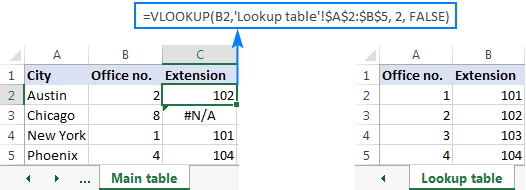
Depending on your business needs, you may want to disguise the error with your own text, zero, or a blank cell.
Example 1. IFERROR with VLOOKUP formula to replace errors with your own text
If you'd like to replace the standard error notation with your custom text, wrap your VLOOKUP formula in IFERROR, and type any text you want in the 2nd argument (value_if_error), for example "Not found":
With the lookup value in B2 in the Main table and the lookup range A2:B4 in the Lookup table, the formula takes the following shape:
=IFERROR(VLOOKUP(B2,'Lookup table'!$A$2:$B$5, 2, FALSE), "Not found")
The screenshot below shows our Excel IFERROR VLOOKUP formula in action:
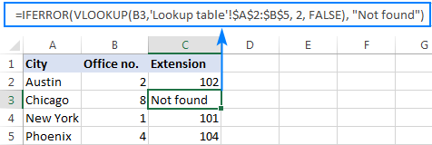
The result looks much more understandable and far less intimidating, isn't it?
In a similar manner, you can use INDEX MATCH together with IFERROR:
=IFERROR(INDEX('Lookup table'!$B$2:$B$5,MATCH(B2,'Lookup table'!$A$2:$A$5,0)), "Not found")
The IFERROR INDEX MATCH formula is especially useful when you want to pull values from a column that lies to the left of the lookup column (left lookup), and return your own text when nothing is found.
Example 2. IFERROR with VLOOKUP to return blank or 0 if nothing is found
If you don't want to show anything when the lookup value is not found, have IFERROR display an empty string (""):
In our example, the formula goes as follows:
=IFERROR(VLOOKUP(B2,'Lookup table'!$A$2:$B$5, 2, FALSE), "")
As you can see, it returns nothing when the lookup value is not in the search list.
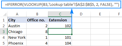
If you'd like to replace the error with the zero value, put 0 in the last argument:
=IFERROR(VLOOKUP(B2,'Lookup table'!$A$2:$B$5, 2, FALSE), 0)
Word of caution! Excel IFERROR function catches all kinds of errors, not only #N/A. Is it good or bad? All depends on your goal. If you want to mask all possible errors, IFERROR Vlookup is the way to go. But it may be an unwise technique in many situations.
For example, if you've created a named range for your table data, and misspelled that name in your Vlookup formula, IFERROR will catch a #NAME? error and replace it with "Not found" or any other text you supply. As the result, you may never know your formula is delivering wrong results unless you spot the typo yourself. In such a case, a more reasonable approach would be trapping only #N/A errors. For this, use IFNA Vlookup formula in Excel 2013 and higher, IF ISNA VLOOKUP in all Excel versions.
The bottom line is: be very careful when choosing a companion for your VLOOKUP formula :)
Nest IFERROR within VLOOKUP to always find something
Imagine the following situation: you look up a specific value in a list and do not find it. What choices do you have? Either get an N/A error or show your own message. Actually, there is a third option - if your primary vlookup stumbles, then search for something else that is definitely there!
Taking our example further, let's create some sort of dashboard for our users that will show them an extension number of a specific office. Something like this:
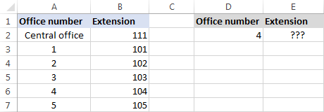
So, how do you pull the extension from column B based on the office number in D2? With this regular Vlookup formula:
=VLOOKUP($D$2,$A$2:$B$7,2,FALSE)
And it will work nicely as long as your users enter a valid number in D2. But what if a user inputs some number that does not exist? In this case, let them call the central office! For this, you embed the above formula in the value argument of IFERROR, and put another Vlookup in the value_if_error argument.
The complete formula is a bit long, but it works perfectly:
=IFERROR(VLOOKUP("office "&$D$2,$A$2:$B$7,2,FALSE),VLOOKUP("central office",$A$2:$B$7,2,FALSE))
If the office number is found, the user gets the corresponding extension number:

If the office number is not found, the central office extension is displayed:

To make the formula a bit more compact, you can use a different approach:
First, check if the number in D2 is present in the lookup column (please notice that we set col_index_num to 1 for the formula to look up and return value from column A): VLOOKUP(D2,$A$2:$B$7,1,FALSE)
If the specified office number is not found, then we search for the string "central office", which is definitely in the lookup list. For this, you wrap the first VLOOKUP in IFERROR and nest this whole combination inside another VLOOKUP function:
=VLOOKUP(IFERROR(VLOOKUP(D2,$A$2:$B$7,1,FALSE),"central office"),$A$2:$B$7,2)
Well, a slightly different formula, the same result:
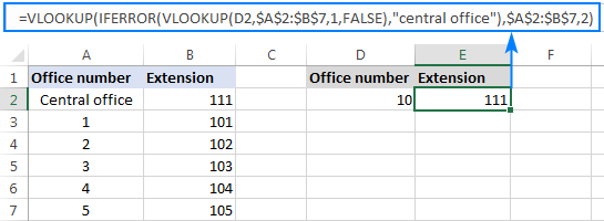
But what is the reason to look up "central office", you may ask me. Why not supply the extension number directly in IFERROR? Because the extension may change at some point in the future. If this happens, you will have to update your data just once in the source table, without worrying about updating each of your VLOOKUP formulas.
How to do sequential VLOOKUPs in Excel
In situations when you need to perform the so-called sequential or chained Vlookups in Excel depending on whether a prior lookup succeeded or failed, nest two or more IFERROR functions to run your Vlookups one by one:
The formula works with the following logic:
If the first VLOOKUP does not find anything, the first IFERROR traps an error and runs another VLOOKUP. If the second VLOOKUP fails, the second IFERROR catches an error and runs the third VLOOKUP, and so on. If all Vlookups stumble, the last IFERROR returns your message.
This nested IFERROR formula is especially useful when you have to Vlookup across multiple sheets as shown in the below example.
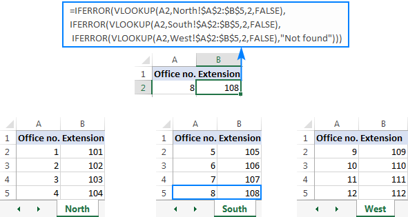
Let's say, you have three lists of homogeneous data in three different worksheets (office numbers in this example), and you want to get an extension for a certain number.
Assuming the lookup value is in cell A2 in the current sheet, and the lookup range is A2:B5 in 3 different worksheets (North, South and West), the following formula works a treat:
=IFERROR(VLOOKUP(A2,North!$A$2:$B$5,2,FALSE), IFERROR(VLOOKUP(A2,South!$A$2:$B$5,2,FALSE), IFERROR(VLOOKUP(A2,West!$A$2:$B$5,2,FALSE),"Not found")))
So, our "chained Vlookups" formula searches in three different sheets in the order we nested them in the formula, and brings the first match it finds:
You can find more examples in this article: VLOOKUP in multiple sheets in Excel.
This is how you use IFERROR with VLOOKUP in Excel. I thank you for reading and hope to see you on our blog next week!
 by
by
89 comments
Hi
I am hoping that you can help me... I am struggling a lot with creating a spreadsheet of data on students marks and obtaining their grade depending on what level test they completed. So...:
Tab 1 - student data with marks:
Mark column 1, standard/ higher test, grade (what I am trying to find out)
Tab 2 - marks and grades
Table 1 - standard test
Mark column 1, grade column 2
Table 2 - higher test
Mark column 1, grade column 2
I require the mark to be obtained from tab 1, along with the column stating either standard or higher test - then obtaining the correct grade from tab 2.
I am hoping you can help me as I have searched everywhere and although I have got an IFERROR function and VLOOKUP I cannot determine how to look up 2 values (mark and test type) and then look at 2 different tables to determine which grade is correct.
So far I have this:
=IFERROR(LOOKUP(D4,'CP7-8'!$A$3:$B$37),0)
But that is just for looking up 1 value and 1 table???
Please please help... confused teacher!
Hello!
I’m sorry but your task is not entirely clear to me. Unfortunately, without seeing your data it is difficult to give you any advice. Please provide me with an example of the source data and the expected result. For me to be able to help you better, please describe your task in more detail.
Please check out the following article on our blog, it’ll be sure to help you with your task: Vlookup multiple matches in Excel with one or more criteria
I am trying to make a formula to check multiple workbooks, I want the formula to check if an item is in column A e.g an egg then check to see if there is an amount in column C e.g 3, if not move on to another workbook to check the same columns. If there is an amount over 1, I want it to say yes and if it is 0 to say no.
Hello!
Sorry, I do not fully understand the task. If you only use one workbook then the formula is -
=IF(AND(A1="egg",C1>3),"Yes","No")
If this is not what you need, please explain your problem in more detail. Give an example of the source data and the expected result.
Hello,
I am trying to do a vlookup function while returning value as below:
1. if blank cell, it will return blank
2. not found, it will return blank
3. if there's a value, it will return the value.
Currently my formula is like this -
=IF(IFERROR(VLOOKUP(E2,A1:B9,2,FALSE),FALSE),(VLOOKUP(E2,A1:B9,2,FALSE)),"")
This formula works only if the value is integer but I encounter an error if the value inside the cell is a string. It will return as this - #VALUE for a string value.
Please help.
Hello!
If I understand your task correctly, the following formula should work for you:
=IF(IFERROR(VLOOKUP(E2,A1:B9,2,FALSE),"")="","", IFERROR(VLOOKUP(E2,A1:B9,2,FALSE),""))
Hope this is what you need.
I am trying to combine two If statements with their own VLookup. I can get it to work if its just one, but not the other. I am using an IF statement to return the data based on the value of cell X, e.g. if cell x = ND, Vlookup to return the value, and if cell x = ED, Vlook up to return the value.
=IF(I6="ND",VLOOKUP(J6,'Post Codes'!A2:B117,2,FALSE),"", IF(I6="ED",VLOOKUP(J6,'Post Codes'!A2:E117,5,False)""))
Please help!
Is there a way to get from which sheet was the value picked up, for example in this case its south, and if there are multiple can it display from what sheets, the value was picked up.
"=IFERROR(VLOOKUP(A2,North!$A$2:$B$5,2,FALSE), IFERROR(VLOOKUP(A2,South!$A$2:$B$5,2,FALSE), IFERROR(VLOOKUP(A2,West!$A$2:$B$5,2,FALSE),"Not found")))"
Hello!
To see how your formula is being executed, you can use the Formula - Evaluate Formula menu item.
This is fantastic stuff, but I have an issue that I cannot seem to get around.. Can you pls pls pls help..
=IFERROR(VLOOKUP($N3245,'GB30'!$A$2:$K$99999,3,FALSE),IFERROR(VLOOKUP($N3245,'GB03'!$A$2:$G$9999,4,FALSE),"DNR"))))))
Looking in 2 sheets for a given value and returning the associated lookup value when it's there. This is working fine, but when a cell is blank I am getting a "Zero" in the result. But I want it to show as an "empty cell" or "". How can these be adapted to result in ""
I have been stuck on this for days!.
Thanks in advance
Jason
Hello!
You can check the obtained values using the IF function:
=IF(IFERROR(VLOOKUP($N3245,’GB30′!$A$2:$K$99999,3,FALSE),IFERROR(VLOOKUP($N3245,’GB03′!$A$2:$G$9999,4,FALSE),”DNR”))))))=0,"",IFERROR(VLOOKUP($N3245,’GB30′!$A$2:$K$99999,3,FALSE),IFERROR(VLOOKUP($N3245,’GB03′!$A$2:$G$9999,4,FALSE),”DNR”)))))))
I hope it’ll be helpful.
Having trouble with the correct IF and VLookup formula. I have 2 separate sheets; 1 with names and the second with names and email addresses. I need a formula that will check to see if the a name on the first sheet is on the second sheet, and if it is, bring over the email address to the first sheet, in a new cell. Any ideas?
Hello!
You need to use a link to another sheet in the VLOOKUP function. Read the instructions on the link.
We have a tool that can solve your task in a couple of clicks: Ablebits Data - Vlookup Wizard.
This tool is available as a part of our Ultimate Suite for Excel that you can install in a trial mode and use for free: https://www.ablebits.com/files/get.php?addin=xl-suite&f=free-trial
Mine worked Perfectly!!!!!!!
Thank you so much for the explanation, very easy to follow. :)
Hi!
I am trying to have my formula look up a text value and if the text is not present then move to the next row under it. If the text is present I want it populate onto a new sheet, if it isn't present then I don't want it to appear at all and I don't want blank rows to populate. Please help. Thanks in advance!
Hello Madi!
What you refer in the first sentence can be done only with the help of VBA.
What you mention further, unfortunately I haven't got what you mean.
Please explain your problem in other words and I’ll try to help you if it is possible.
=IFERROR(VLOOKUP(A2,'Balance'!A:C,2,FALSE),0) is not working when A2 more than A999 how to solve it
Hello!
I have checked the work of your VLOOKUP function in my own file and haven’t found any error. However, the formula I used looks as follows:
=IFERROR(VLOOKUP(A2,[’Balance’]Sheet1!A:C,2,FALSE),0)
May this be the problem? If you are still getting an error, please describe the problem in more detail so that I’ll be able to help you better.
when we revise the VLOOKUP Function, what is replaced with COLUMN Function
I'm using excel office 360. When I do the vlookup, am getting the return value of the "text formula I typed in". How to fix this?
Hello Mam,
Please send me a video of IFERROR formula with vlookup.
Ablebits is the best excel adviser, appreciated your job
Regard,
you are my number one !!!
Please send me main excel accounting formulas at above email
Hi, mam
I have a data in sheet first is name and second is dob i want to do if month is coming dob highlights automatically
Column A2:A173 contains 1,2 or is blank
column c contains a date or is blank
I need a formula to do the following:
If column a contains a 1 or 2 look at the same row in column C and if that contains ANY entry (will most likely be a date) count it.
Your timing is excellent. Just started new job and they gave me 3 files with 1 million rows each. Of couse split amongst tabs. I was going crazy with all the vlookup and now you helped me save hours of work. Thank you thank you.
Hi
Is there a way i can get a cell to return a blank cell after a particular date? if its before a date then use zero. Im having trouble with so many commands.