From this short tutorial you'll learn about the new IFS function and see how it simplifies writing nested IF in Excel. You'll also find its syntax and a couple of use cases with examples.
Nested IF in Excel is commonly used when you want to evaluate situations that have more than two possible outcomes. A command created by nested IF would resemble "IF(IF(IF()))". However this old method can be challenging and time consuming at times.
The Excel team has recently introduced the IFS function that is likely to become your new favorite one. Excel IFS function is available only in Excel 365, Excel 2021 and Excel 2019.
The Excel IFS function - description and syntax
The IFS function in Excel shows whether one or more conditions are observed and returns a value that meets the first TRUE condition. IFS is an alternative of Excel multiple IF statements and it is much easier to read in case of several conditions.
Here's how the function looks like:
It has 2 required and 2 optional arguments.
- logical_test1 is the required argument. It's the condition that evaluates to TRUE or FALSE.
- value_if_true1 is the second required argument that shows the result to be returned if logical_test1 evaluates to TRUE. It can be empty, if necessary.
- logical_test2…logical_test127 is an optional condition that evaluates to TRUE or FALSE.
- value_if_true2…value_if_true127 is an optional argument for the result to be returned if logical_testN evaluates to TRUE. Each value_if_trueN relates to a condition logical_testN. It can also be empty.
Excel IFS lets you evaluate up to 127 different conditions. If a logical_test argument doesn't have certain value_if_true, the function displays the message "You've entered too few arguments for this function". If a logical_test argument is evaluated and corresponds to a value other than TRUE or FALSE, IFS in Excel returns the #VALUE! error. With no TRUE conditions found, it shows #N/A.
The IFS function vs. nested IF in Excel with use cases
The benefit of using the new Excel IFS is that you can enter a series of conditions in a single function. Each condition is followed by the result that will be used if the condition is true making it straightforward to write and read the formula.
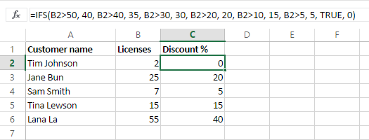
Let's say you want to get the discount according to the number of licenses the user already has. Using the IFS function, it will be something like this:
=IFS(B2>50, 40, B2>40, 35, B2>30, 30, B2>20, 20, B2>10, 15, B2>5, 5, TRUE, 0)

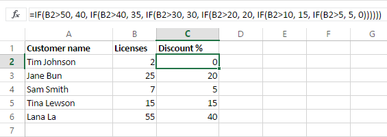
Here's how it looks with nested IF in Excel:
=IF(B2>50, 40, IF(B2>40, 35, IF(B2>30, 30, IF(B2>20, 20, IF(B2>10, 15, IF(B2>5, 5, 0))))))

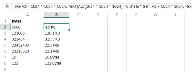
The IFS function below is easier to write and update than its Excel multiple IF equivalent.
=IFS(A2>=1024 * 1024 * 1024, TEXT(A2/(1024 * 1024 * 1024), "0.0") & " GB", A2>=1024 * 1024, TEXT(A2/(1024 * 1024), "0.0") & " Mb", A2>=1024, TEXT(A2/1024, "0.0") & " Kb", TRUE, TEXT(A2, "0") & " bytes")

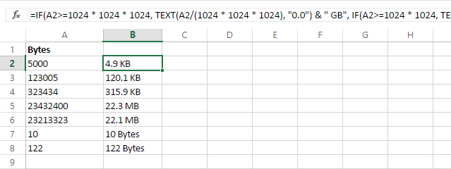
=IF(A2>=1024 * 1024 * 1024, TEXT(A2/(1024 * 1024 * 1024), "0.0") & " GB", IF(A2>=1024 * 1024, TEXT(A2/(1024 * 1024), "0.0") & " Mb", IF(A2>=1024, TEXT(A2/1024, "0.0") & " Kb", TEXT(A2, "0") & " bytes")))

 by
by
70 comments
The IFS function is actually sometimes worse than even some of the posters point out. I wrote a recursive function that called itself within an IFS statement (if certain boundary conditions such as out of range etc. were met, exit gracefully, but in the base case, recursively call the Lambda function). I wracked my brains for a long time trying to figure out why I continued to get a #Value error, strongly suspecting that I was running into an infinite loop. Then I read a post that IFS evaluates ALL conditions even if it only executes the first TRUE condition, and rewrote the IFS to include a nested IF only for the recursive call. The program worked fine. Microsoft seems to have improperly documented this but it is likely a common way to get hung up in recursion.
Can you please help to write if (and nested formula for following conditions?
IF TAXABLE INCOME IS OVER: BUT NOT OVER: THE TAX IS:
$0 $23,200 10% of taxable income
$23,200 $94,300 $2,320 + 12% of the amount over $23,200
$94,300 $201,050 $10,852 + 22% of the amount over $94,300
$201,050 $383,900 $34,337+ 24% of the amount over $201,050
$383,900 $487,450 $78,221 + 32% of the amount over $383,900
$487,450 $731,200 $111,357 + 35% of the amount over $487,450
$731,200 No limit $196,669 + 37 % of the amount over $731,200
Hi! All the necessary information is in the article above. For example:
=IFS(A1>731200,A1*0.37,A1>487450,111357+(A1-487450))
You can also find useful information in this article: Excel Nested IF statements - examples, best practices and alternatives.
=IF(A3=0,AVERAGE(A2:B2),IF(A4=0, Averge(A2:B3), AVERAGE(A2:B4)))
A B
1 2
3 0
0 0
Result= #NAME?
What is wrong in formula?
Hi! Your formula contains no errors. AVERAGE function is available in all versions of Excel since 2007. It is possible that there is a #NAME error in one of the cells that is referenced by this formula.
You can also find useful information in this article: #NAME error in Excel: reasons and fixes.
I am trying to write formula that if the value $K$7="ABC", and value in L16 is less than 45, it should show amount 45. If value returned in L16 is greater that 45, it should return the value whatever is in L16
AND
Similarly if the value $K$7="XYZ", and value in L16 is less than 2, it should show amount 2. If value returned in L16 is greater that 2, it should return the value whatever is in L16.
what formula can I use. Can't get my head around it, its driving me nuts.
I am using below formula now but it is not giving correct figure. Tried IFS and CONCATENATE but didn't work for me either.
=IF(AND($K$7="JNFX", L16<40), 45, L16)+IF(AND($K$7="SATCHEL", L16<2), 0, 0)+IF(AND($K$7="JNFX", L16<40), 0, 0)+ IF(AND($K$7="SATCHEL", L16<2), 2, L16)
HELP!!!
Hi! If I understand your task correctly, the following tutorial should help: Nested IF in Excel – formula with multiple conditions.
=IF(K7="ABC",IF(L16<45,45,L16), IF(K7="XYZ",IF(L16<2,2,L16),""))
hi, i have a question, my formula as stated =IFS(F17>=5,F17/2,F1714,"7")
if we work more than 5 year in the company, add'l 2.5 days entitle and add'l leave only up to 7 days , its mean if you work more than 14 year only can get up to 7 days additional leave.
=IFS(F17>=5,F17/2,F1714,"7") is formula will show if work than 14 year it will give me the answer more than 7 days as the 1st logical test was put more than 5 year mean also included 14 year.. so how i need to modify my formula.
thank in advance for your help!
sorry amend my formula: =IFS(F2>=5,F2/2,F214,"7")
why my formula keep changing with i copy ouT from my file.
this is correct : IFS (F2>=5,F2/2,F214,"7")
Hi! If I understand the problem correctly, the first condition in the formula includes the second condition.
Therefore, either supplement the first condition or change the order in which the conditions are checked.
=IFS(AND(F2>=5,F2<14),F2/2,F2>=14,7)
=IFS(F2>=14,7,F2>=5,F2/2)
thanks very much sir!
Am trying to find the best formula to spread a quantity (total sales) between 2 dates with a prorated value per year in between.
I suppose I need a combinations of IFS. So far, I could only do this manually. But this would get extremely time-consuming if I had 200+ rows.
My focus is which IFS formula can help me calculate the values from H9:M17 ?
Your task is not completely clear to me. Please clarify your specific problem or provide additional information to understand what you need. Provide me with an example of the source data and the expected result.
I am trying to write the following formula:
=IFS(J19="Monday",B15,J19="Tuesday",C15,J19="Wednesday",D15,J19="Thursday",E15,J19="Friday",F15)
The formula works if I type the day in cell J19, but J19 contains a formula which returns the specific day, which the above formula does not seem to read?
How can I guess what formula you are using in cell J19, what value it returns, and what value you are writing to that cell?
the formula in J19 is =IF(H19,H19,"") . It is just needed to return the day of whatever date is entered in H19.
To return the day of any date, use the DAY function.
I am working on a nested IF statement that looks at a start date and end dates, compares it to a column date and places a letter in the cell if that cell falls between the dates. I have read that the IF statements are not able to determine dates? How can I fix this in my nested if statement?
Currently I have 8 nested if statements that read IF(start date >= cell date, end date<=cell date,"L"), if not than blank""
The formula is working, but it is not right. wondering if the dates are not being read correctly. Any advice?
Hi! From your description, it is difficult to understand the problem. I can guess that some dates are written as text. Try these instructions: How to convert text to date in Excel.
IFS(), as it is presently implemented in Excel, has a significant drawback. IFS(logical1,expr1,logical2,expr2,logical3,expr3,TRUE, default expr ) always evaluates all of the logicals and all of the expressions. The corresponding nested IF(logical1,expr1,IF(logical2,expr2,IF(logical3,expr3,default expr ) ) ) will always evaluate logical1, but will only evaluate expr1 when logical1 is true, and will only evaluate logical2, when logical 1 is false, etc.
IFS() does not return errors from logical tests that would never be reached by the nested IF() form, and does not return errors from expressions that would never be evaluated by the nested IF() form.
IFS() will perform time consuming operations like table lookups and data queries that would never be reached by the nested IF() form.
IFS() will return #NA when none of the logical expressions was true. When logical1, logical2, and logical3 are all false.,
IFS(logical1,expr1,logical2,expr2,logical3,expr3) returns #NA
IF(logical1,expr1,IF(logical2,expr2,IF(logical3,expr3) ) ) returns FALSE
I'm sure the rational for choosing the present implementation was along the lines of "it corresponds to evaluating a vector expression", or "it corresponds to modern CPU architectures that perform speculative execution", "it allows for parallel execution on multiple cores". That these rationales also consume more CPU cycles and drive new hardware purchases that require a new OS license and a new Office license is an example of (un) natural selection. None of the rationales is valid. Speculative evaluation of nested IF() functions could also be scheduled on multiple cores for parallel execution.
Until Microsoft rewrites the IFS() function, using ctrl-enter to write
=IF(logical1,expr1,
IF(logical2,expr2,
IF(logical3,expr3,
default )))
has enough advantages over
=IFS(logical1,expr1,
logical2,expr2,
logical3,expr3,
TRUE. default )
to continue using nested IF() instead of IFS()
THANK YOU FOR THIS COMMENT!
I have been losing my mind trying to figure out why my IFS functions are evaluating all the conditions when nested IFS do not. This is an incredible oversight and has major performance issues for people with large or complex tables/worksheets (my particular case uses UDFs with nested IFS for error handling).
It really boggles the mind why they would make IFS function without the short-circuit ability built into the IF statement.
I have a file with multiple tabs. I need to have information read from one tab to a roll up tab. The one tab has a question that can be answered YES, NO or N/A. The questions are answered by an X in the appropriate column. I need the answer to read to the roll up sheet as Yes or No or N/A depending on where the X was placed on the question in the tab.
Tab 1
Question Audits completed Yes No N/A
X
Roll up
Audits Completed Yes
Hi!
If I understand your task correctly, try the following formula:
=IF(VLOOKUP(Sheet2!A1,'tab1'!A2:D20,2,FALSE)="x","yes", IF(VLOOKUP(Sheet2!A1,'tab1'!A2:D20,3,FALSE)="x","no", IF(VLOOKUP(Sheet2!A1,'tab1'!A2:D20,4,FALSE)="x","N/A","")))
The following tutorial should help: IF VLOOKUP in Excel: Vlookup formula with If condition.
Which formula need to used for calculating the commission for different seller vendor with different Rate complexity e.g.
Vendor list....
Vendor Name Sell Commission
A 2000
B 5000
C 10000
D 6000
Vendor
Name Percentage Flat Rate in Rs.
A 10% OR 500 Whichever is low
B 5%
C 400
D 15% 200 Whichever is low
Hi!
To find the smaller number, use the MIN function.
For example, MIN(A1*10%, 500)
My query is how to calculate the commission on sale with provided commission table.
If I understand correctly, you have a separate commission for each vendor. Write down 4 formulas.
MIN(A1*10%, 500)
A2*5%. ....
etc.
Hi Alexander,
Need one single formula by which I can calculate all categories vendor transaction commission.
Thank you for your support.
Regards,
Datta
Hi! You can combine formulas with a nested IF formula. For example:
=IF(A2="A",MIN(B2*0.1,500),IF(A2="B",B2*0.05,""))
Trying to get this IFS statement to work. Seems simple enough but I seem to be missing something. I can get the result for the first statement or the third statement but not the second statement Middle). =IFS(K33L33,2,K33>L33,3)
=IFS(L33<K33,3,"L33+5"K33,1)
Hi!
The expression "L33+5"K33 does not make sense. Perhaps L33+5=K33 ?
Please read the above article carefully.
Hello,
I'm trying to get the following formula to work but this message keeps showing: "You've entered too few arguments for this function."
The formula in question: *the excel software is programmed to be in french so SI.CONDITIONS translates to IFS*
=SI.CONDITIONS(C20="Anglais 1"; 134-104; C20="Anglais 2"; 134-204; C20="Anglais 3"; 134-304; C20="Anglais 4"; 134-404; C20="Anglais 5"; 134-504; C20="Arts Plastiques 4"; 168-402; C20="Arts Plastiques 5"; 168-502; C20="Chimie 5"; 051-504; C20="Éducation Financière"; 102-522; C20="Espagnol"; 141-514;"0")
I know in this article, it states that if that specific message appears it is because I never put a value_if_true. But I think I did, but now I'm not too sure. Is it because my values have a dash ?
Please someone help me haha
Hello!
Use double quotes. Instead of 134-104, write "134-104" and so on.
Hello,
I tried using the double quotes as you suggested and the same message keeps appearing. Should I consider doing another formula ?
IT WORKED !! I'm so happy haha Turns out that I had to eliminate the "0" value at the end and replace it with the end of my parenthesis. Thank you so much for your help !!
Hi, I want to build a couple of formulas for current and previous month scores based on a table of data. Basically, if today's date is in the month of x (shown in column A), then display a specific score from column B.
In A2:A13, I have the names of the month's of the year.
In B2:B13, I have scores that are totals for that given month.
In D1, I want to display the current month's score based on today's date.
In D2, I want to display the previous month's score based on today's date.
I know it involved an IFS statement using TODAY(), and the appropriate cell in column B not being blank, and I'm at a loss on how to put it all together.
Hello!
If I understand your task correctly, the following formula should work for you:
=SUMIF(A2:A13,TEXT(TODAY(),"mmmm"),B2:B13)
Hope this is what you need.
Thanks Alexander, very close.
I'm looking to show the specific score for the corresponding month, not the sum of the scores.
So if A11's value is October, and Todays date is October 31st, show the value in B11
Hello!
Have you tried using a formula? If your data contains only one cell "October", then you will get the score for October.
You can also use the VLOOKUP function to find the value:
=VLOOKUP(TEXT(TODAY(),"mmmm"),A2:B13,2,FALSE)
Hi, I hope you can help me. I am looking for a formula that will calculate the date range between cells, (NETWORKDAYS, no holidays), where the cells used in the date range will depend if the are populated.
The calculation needs to consider the following:
C1 is the end date, and the start date is either B1 or A1.
B1 is the first start date to look at. If B1 is populated, then calculate the "networkdays" between B1 & C1.
If B1 is blank, then calculate the "networkdays" between A1 & C1.
If C1 is blank, the cell should be blank, even if A1 and B1 are populated.
This is what I have, and it works until C1 is blank:
=IF(B1="",NETWORKDAYS(A1,C1),NETWORKDAYS(B1,C1)))
Hello!
If I understand correctly, add another nested condition to the IF formula:
=IF(C1<>"",IF(B1="",NETWORKDAYS(A1,C1),NETWORKDAYS(B1,C1)),"")
Thank you very much, Alexander, it works (with the addition one an extra closed parenthesis).
Hi, I'm trying to write formula that will return "BH" if cell contains "Brighton" and "LDN" if cell contains "London".
It woks only for cells wit "Brighton", but not cells with London and I'm getting #VALUE! error.
=IFS(SEARCH("Brighton",C48691),"BH",SEARCH("London",C48691),"LDN")
Thank you.
Aga
Hello!
Use the ISNUMBER function to prevent errors from occurring.
=IFS(ISNUMBER(SEARCH(“Brighton”,C48691)),”BH”,ISNUMBER(SEARCH(“London”,C48691)),”LDN”)
Thank you. I tried your formula, but now I'm getting #N/A error in both cases
Hi!
Check the quotes in your formula. Change ” to "
Hi!
I didn't notice it. Thank you very much for your help. That's great.
So the error was I didn't properly research how to formulate looking for "TRUE" statements. The "TRUE" in the formulas need to be without quotes.
Hello all,
I have a very long IFS() statement that I'm trying to get to work for a personal project to randomly generate a first name given three different criteria (all three of which are also randomly generated).
It's always returns the #N/A error, which I know is because it finds no "TRUE" statements. I've confirmed this by looking at both "Show Calculation Steps" and "Evaluate Formula" which shows the formula is properly randomly generating a name from each column. But they are all preceded by "FALSE," telling me that it's not recognizing any of the randomly generated criteria in the first place.
Here is an example of the recurring arguments I've put in to account for every outcome:
IFS(...,AND(AA22="Roman",X22="*",Z22="Female")="TRUE",VLOOKUP(RANDBETWEEN(1,50),RaceFirstName[#All],53),...)
AA=First Name's Origin [=VLOOKUP(RANDBETWEEN(1,100),RaceFirstName[#All],3)]
X=Race [=VLOOKUP(RANDBETWEEN(1,100),RaceFirstName[#All],2)]
Z=Gender [=VLOOKUP(RANDBETWEEN(1,2),Gender[#All],2)]
The VLOOKUP is looking at a large table and randomly selecting a name from there.
I've gone through the "RaceFirstName" and "Gender" tables to make sure there was no space at the end or beginning (as that's an issue I've found to be common).
The only three issues I can think of is
1. that the colums X, Z, and AA are still viewed as formulas and not values by the IFS() statement.
2. that the order of the references need to be X, Z, AA and not as they are now (currently not in that order)
3. that the formula itself has too many conditions (it has about 60 conditions, but maybe due to the AND statements, it's too much for it to want to calculate)
Any help or insight would be most welcome. Hopefully I was clear enough.
Thank you so much for taking the time to read this.
Thank you for taking the time to read this.
I would like to use IF to update a value in another field (that currently has a value). I am not sure how to enter just the current time.
=if(c2="x",b1=Now)
Ideally, someone makes c2 = x and then this happens. I don't know how to run a formula in the current field without overwriting the formula.
Thanks
Hello!
If a value is written in a cell, then it is impossible to change it using a standard Excel formula. You need to use a VBA macro.
I'm trying to write a formula that will analyze whether win, lose or tie a golf whole. I needs to consider the difference in player handicaps (me 2, competitor 11), the rating of the hole (7) and the 2 scores made on the whole (me 4, him 5), then return a -1 for a loss, a 0 for a tie or a +1 for a win. Example, I have to give my opponent 9 strokes, the distribution of which is determined by the rating of each hole. Hole 1 is rated #7 so he gets a stroke there. If I score 4 and he scores 5, we tie because 5-1 = 4. If I make 4 and he makes 6, I win because 6-1=5 which is higher than 4. If we both score 4, he wins because his 4-1 beats my 4. How can I do this?