The tutorial explains the specificities of the SUBTOTAL function in Excel and shows how to use Subtotal formulas to summarize data in visible cells.
In the previous article, we discussed an automatic way to insert subtotals in Excel by using the Subtotal feature. Today, you will learn how to write Subtotal formulas on your own and what advantages this gives to you.
Excel Subtotal function - syntax and uses
Microsoft defines Excel SUBTOTAL as the function that returns a subtotal in a list or database. In this context, "subtotal" is not just totaling numbers in a defined range of cells. Unlike other Excel functions that are designed to do only one specific thing, SUBTOTAL is amazingly versatile - it can perform different arithmetic and logical operations such as counting cells, calculating average, finding the minimum or maximum value, and more.
The SUBTOTAL function is available in all versions of Excel 2016, Excel 2013, Excel 2010, Excel 2007, and lower.
The syntax of the Excel SUBTOTAL function is as follows:
Where:
- Function_num - a number that specifies which function to use for the subtotal.
- Ref1, Ref2, … - one or more cells or ranges to subtotal. The first ref argument is required, others (up to 254) are optional.
The function_num argument can belong to one of the following sets:
- 1 - 11 ignore filtered-out cells, but include manually hidden rows.
- 101 - 111 ignore all hidden cells - filtered out and hidden manually.
| Function_num | Function | Description | |
| 1 | 101 | AVERAGE | Returns the average of numbers. |
| 2 | 102 | COUNT | Counts cells that contain numeric values. |
| 3 | 103 | COUNTA | Counts non-empty cells. |
| 4 | 104 | MAX | Returns the largest value. |
| 5 | 105 | MIN | Returns the smallest value. |
| 6 | 106 | PRODUCT | Calculates the product of cells. |
| 7 | 107 | STDEV | Returns the standard deviation of a population based on a sample of numbers. |
| 8 | 108 | STDEVP | Returns the standard deviation based on an entire population of numbers. |
| 9 | 109 | SUM | Adds up the numbers. |
| 10 | 110 | VAR | Estimates the variance of a population based on a sample of numbers. |
| 11 | 111 | VARP | Estimates the variance of a population based on an entire population of numbers. |
In fact, there is no need to memorize all function numbers. As soon as you start typing a Subtotal formula in a cell or in the formula bar, Microsoft Excel will display a list of available function numbers for you.
For example, this is how you can make a Subtotal 9 formula to sum up the values in cells C2 to C8:
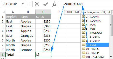
To add a function number to the formula, double-click on it, then type a comma, specify a range, type the closing parenthesis, and press Enter. The completed formula will look like this:
=SUBTOTAL(9,C2:C8)
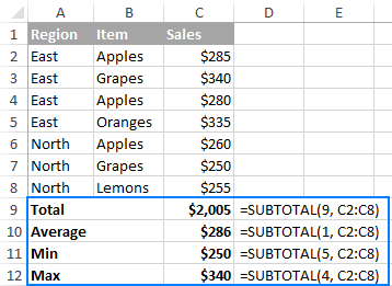
In a similar manner, you can write a Subtotal 1 formula to get an average, Subtotal 2 to count cells with numbers, Subtotal 3 to count non-blanks, and so on. The following screenshot shows a few other formulas in action:
Note. When you use a Subtotal formula with a summary function like SUM or AVERAGE, it calculates only cells with numbers ignoring blanks and cells containing non-numeric values.
Now that you know how to create a Subtotal formula in Excel, the main question is - why would one want to take the trouble of learning it? Why not simply use a regular function like SUM, COUNT, MAX, etc.? You will find the answer right below.
Top 3 reasons to use SUBTOTAL in Excel
Compared to the traditional Excel functions, SUBTOTAL gives you the following important advantages.
1. Calculate values in filtered rows
Because the Excel SUBTOTAL function ignores values in filtered-out rows, you can use it to create a dynamic data summary where subtotal values are re-calculated automatically according to the filter.
For example, if we filter the table to show sales only for the East region, the Subtotal formula will automatically adjust so that all other regions are removed from the total:
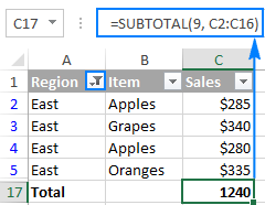
Note. Because both function number sets (1-11 and 101-111) ignore filtered out cells, you can use ether Subtotal 9 or Subtotal 109 formula in this case.
2. Calculate only visible cells
As you remember, Subtotal formulas with function_num 101 to 111 ignore all hidden cells - filtered out and hidden manually. So, when you use Excel's Hide feature to remove irrelevant data from view, use function number 101-111 to exclude values in hidden rows from subtotals.
The following example will help you gain more understanding of how it works: Subtotal 9 vs. Subtotal 109.
3. Ignore values in nested Subtotal formulas
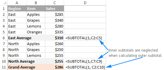
If the range supplied to your Excel Subtotal formula contains any other Subtotal formulas, those nested subtotals will be ignored, so the same numbers won't be calculated twice. Awesome, isn't it?
In the screenshot below, the Grand Average formula SUBTOTAL(1, C2:C10) ignores the results of the Subtotal formulas in cells C3 and C10, as if you used an Average formula with 2 separate ranges AVERAGE(C2:C5, C7:C9).
Using Subtotal in Excel - formula examples
When you first encounter SUBTOTAL, it may seem complex, tricky, and even pointless. But once you get down to brass tacks, you will realize that it's not that difficult to master. The following examples will show you a couple of helpful tips and inspirational ideas.
Example 1. Subtotal 9 vs. Subtotal 109
As you already know, Excel SUBTOTAL accepts 2 sets of functions numbers: 1-11 and 101-111. Both sets ignore filtered-out rows, but numbers 1-11 include manually hidden rows whereas 101-111 exclude them. To better understand the difference, let's consider the following example.
To total filtered rows, you can use either Subtotal 9 or Subtotal 109 formula like shown in the screenshot below:
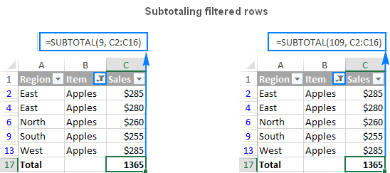
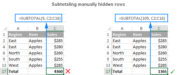
But if have hidden irrelevant items manually by using the Hide Rows command on the Home tab > Cells group > Format > Hide & Unhide, or by right clicking the rows, and then clicking Hide, and now you want to total values only in visible rows, Subtotal 109 is the only option:
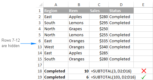
Other function numbers work in the same way. For example, to count non-blank filtered cells, either Subtotal 3 or Subtotal 103 formula will do. But only Subtotal 103 can properly count visible non-blanks if there are any hidden rows in the range:
Note. The Excel SUBTOTAL function with function_num 101-111 neglects values in hidden rows, but not in hidden columns. For example, if you use a formula like SUBTOTAL(109, A1:E1) to sum numbers in a horizontal range, hiding a column won't affect the subtotal.
Example 2. IF + SUBTOTAL to dynamically summarize data
If you are creating a summary report or a dashboard where you have to display various data summary but you don't have space for everything, the following approach might be a solution:
- In one cell, make a drop-down list containing the functions names such as Total, Max, Min, and so on.
- In a cell next to the dropdown, enter a nested IF formula with the embedded Subtotal functions corresponding to the function names in the drop-down list.
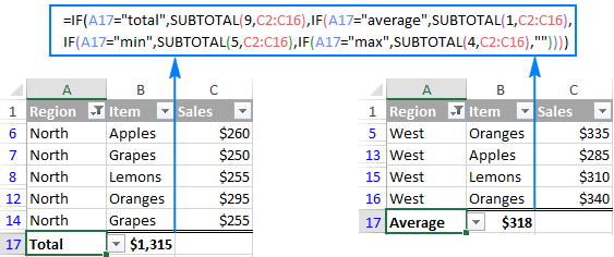
For example, assuming the values to subtotal are in cells C2:C16, and the drop-down list in A17 contains Total, Average, Max, and Min items, the "dynamic" Subtotal formula is as follows:
=IF(A17="total", SUBTOTAL(9,C2:C16), IF(A17="average", SUBTOTAL(1,C2:C16), IF(A17="min", SUBTOTAL(5,C2:C16), IF(A17="max", SUBTOTAL(4,C2:C16),""))))
And now, depending on what function your user selects from the drop-down list, the corresponding Subtotal function will calculate values in filtered rows:
Tip. If all of a sudden the drop-down list and the formula cell disappear from your worksheet, be sure to select them in the filter list.
Excel Subtotal not working - common errors
If your Subtotal formula returns an error, it's likely to be because of one of the following reasons:
#VALUE! - the function_num argument is other than an integer between 1 - 11 or 101 - 111; or any of the ref arguments contains a 3-D reference.
#DIV/0! - occurs if a specified summary function has to perform a division by zero (e.g. calculating an average or standard deviation for a range of cells that does not contain a single numeric value).
#NAME? - the name of the Subtotal function is misspelled - the easier error to fix :)
Tip. If you don't feel comfortable with the SUBTOTAL function yet, you can use the built-in SUBTOTAL feature and have the formulas inserted for you automatically.
That's how to use the SUBTOTAL formulas in Excel to calculate data in visible cells. To make the examples easier to follow, you are welcome to download our samples workbook below. Thank you for reading!
Practice workbook
Excel SUBTOTAL formula examples (.xlsx file)
 by
by
33 comments
Hello,
Can we do subtotal for negative values only or positive values?
Regards,
M
Hi! Apply filters to your dataset (you can use the keyboard shortcut Ctrl + Shift + L).
Filter the relevant column to show only positive or only negative numbers.
Use the formula:
=SUBTOTAL(109,B2:B50)
Remember to adjust the range (B2:B50) according to your actual data.
You can also use the SUMIF function to find the sum of only positive values or only negative values:
=SUMIF(B2:B50,">=0",B2:B50)
Instead of a Range, can a formula be used? I'm just balancing my checkbook. I take the current balance, plus add the new deposit and deduct a withdrawal. for example: Col A consists of the deposits. Col B consist of the withdrawals. C is the balance in the account. the formula in each cell references the cell above, plus the deposit, less the withdrawal =SUM(C1+A2 - B2). However, I'm filtering and hiding some rows, so I would like the calculation to occur only with the visible cells. I typed =Subtotal(9, C1+A2-B2). that doesn't work. Is there a way to do what I'm trying to do?
Hello!
The Excel functions you are using cannot ignore hidden cells. Try AGGREGATE function which can ignore hidden rows.
I am working with a table and I am wanting to get dynamic averages with different level of outliers excluded. Ultimately I would like a full average, 1 standard deviation average, and 2 standard deviation average.
In the table I have filters that let me select what I want available for the data set such as character, potara, and others. I have used subtotal to get the average and the standard deviation, but I have not been able to create the other two.
Subtotal cell average 51567
Subtotal cell standard deviation 26697.70
List of values come from:
28680, 82900, 83610, 31100, 27200, 55910
DATA PAGE
CODE PRODUCT UNIT SALE QTY
A125 POTATO Nos 12
C365 ONION Nos 25
A125 POTATO Bxs 2
V254 TOMATO Bxs 1
1254 CHILLY Nos 36
C365 ONION Bxs 3
A125 POTATO Nos 7
C365 ONION Nos 14
A125 POTATO Bxs 1
V254 TOMATO Bxs 3
1254 CHILLY Nos 24
C365 ONION Bxs 1
129
RESULT PAGE
CODE PRODUCT UNIT TOTAL SALE QTY
A125 POTATO Nos 19
C365 ONION Nos 39
A125 POTATO Bxs 3
V254 TOMATO Bxs 4
1254 CHILLY Nos 60
C365 ONION Bxs 4
129
* here Quantity summerized
which formula using to get automatically total sale value, if code,product & unit columns are matching
Hello!
If I understand the question correctly, you can use the SUMIFS function to calculate the sum of matching cells.
i have very simple problem
ITEM PRICE
ORANGE 10
APPLE 25
APPLE 30
CHERRY 90
i want to get the maximum Price of each subgroup at each change in Item
i know this is very easy to get with Excel's built-in Subtotal function,
but the Excel Subtotal function introduces new rows to show the reults.
Is it possible to write a Subtotal function to do this and not introduce additional rows?
can this be done without a Macro or VBA?
Secondly, how to access these results to put into cells of a new table on a new worksheet?
I do not have any known values to "lookup" or "match".
Hello!
Please check out the following article on our blog, it’ll be sure to help you with your task: Excel MAXIFS function - get largest value based on multiple criteria
Hope this is what you need.
How to calculate std.dev subtotal?
I am getting it wrong.
I am having trouble getting the cell subtotals c7:c16 for total
1267X9= IN EXCEL
2219X2=
204.65X50=
SUB-TOTAL
Please advise how do I count similar text with subtotal 109, range, ???
Thanks !
Hello Prathap!
For me to be able to help you better, please describe your task in more detail. It’ll help me understand it better and find a solution for you. Thank you.
Hi,
Loving this formula but having a small issue with it.
Can you please let me know if it doesn't work on dates or if I am doing something wrong?
Cheers
This didn't really answer my concern. I am using a SUMIF function over a large amount of data. I also need to filter the data for multiple variables. The data set has history stacked based on changes in an item/upc# there are thousands of upc# per year
2017 TOTAL of ALL upc#s (using SUMIF function)
2018 TOTAL of ALL upc#s (using SUMIF function)
2019 TOTAL of of ALL upc#s (using SUMIF function)
I would like to see the subtotal for each of the years based on what criteria I have filtered. Since I am using the SUMIF to get the totals values do not change based on filter selection. I need a way to combine the SUMIF function with a SUBTOTAL so that total is representative of the criteria I have filtered
My Query:
Date Name Qty Sales Amount Received Amount "Balance Amount"
1-Jul-19 A 100 1,000 100 900
2-Jul-19 B 200 2,000 200 2700
3-Jul-19 E 250 2,500 250 4950
3-Jul-19 A 300 3,000 300 7650
3-Jul-19 E 150 1,500 150 9000
4-Jul-19 B 180 1,800 200 10600
4-Jul-19 A 120 1,200 1500 10300
5-Jul-19 C 130 1,300 1000 10600
6-Jul-19 C 220 2,200 3000 9800
I want Subtotal formula in Balance Side. Whenever I filter by name It automatically show me his (+) or (-) balance as per Name.
Kindly suggest or send me email with solution.
Thanks
How to calculate through subtotal formula
Credit Note for April'18 to Nov'18 SPP Hills
Month Total Penalty Zone Site Count Penalty/Site Zone wise Penalty
April'18 141288.00 NB 112 537.22 60168.27
April'18 Sikkim 151 537.22 81119.73
May'18 152513.00 NB 123 527.73 64910.38
May'18 Sikkim 166 527.73 87602.62
June'18 89684.00 NB 123 311.40 38302.54
June'18 Sikkim 165 311.40 51381.46
July'18 254329.00 NB 123 883.09 108619.68
July'18 Sikkim 165 883.09 145709.32
August'18 198451.00 NB 124 689.07 85444.18
August'18 Sikkim 164 689.07 113006.82
Sep'18 62809.00 NB 123 218.09 26824.68
Sep'18 Sikkim 165 218.09 35984.32
Oct'18 113675.00 NB 123 394.70 48548.70
Oct'18 Sikkim 165 394.70 65126.30
Nov'18 199150.00 NB 122 691.49 84362.15
Nov'18 Sikkim 166 691.49 114787.85
1211899.00 2280 1211899.00
Zone Avg Site Count Avg Penalty/Site Zone wise Penalty
North Bengal ??? ??? 517180.58
Sikkim ??? ??? 694718.42
Hi!
no doubt it is a very easily approachable to understand how to use subtotal formula for filtering data in sheet. i really liked the coordination between the given example and explanation in details . I hope you will let us explore the excel to do more better
Dear Sir,
I need subtotal formula.
Example
SECTION(MM) TOTALWT(KG.)
MS L65X65X5 PG 805.10
MS L65X65X5 PG 805.10
MS L65X65X5 PG 805.10
MS L65X65X5 PG 805.10
MS L45X45X5 PG 1579.78
MS L45X45X5 PG 1184.83
MS L50X50X5 PG 109.44
MS L50X50X5 PG 134.98
MS L45X45X5 PG 120.77
MSPLT 12 1130.40
MSPLT 12 407.04
MSPLT 06 102.91
MSPLT 06 102.91
MS L65X65X6 PG 36.19
MS L65X65X6 PG 36.19
MS L50X50X5 PG 145.92
MS L45X45X5= ?
MS L50X50X5= ?
MS L65X65X5= ?
MS L65X65X6= ?
MSPLT 06= ?
MSPLT 12= ?
MS L45X45X5 Total 2,885.38
MS L50X50X5 Total 390.34
MS L65X65X5 Total 3,220.40
MS L65X65X6 Total 72.38
MSPLT 06 Total 205.82
MSPLT 12 Total 1,537.44
Grand Total 8,311.76
I want to be able to do a countA subtotal on cells that also have formulas. Currently it is counting the cells that have the formulas even though they do not have the designated values I am looking for.
Thanks
I want to be able to do a countA subtotal on cells that also have formulas. Currently it is counting the cells that have the filters even though they do not have the designated values I am looking for.
Thanks
Hi,
I want to learn how subtotal function is used more than one range.How is it work.Can you send example so i learn easily.
Thanking you
Thanks very much for sharing this information, this is a really detailed tutorial. I haven't been using Excel for a very long time so still trying to navigate my way around it. It has been a really useful piece of software for me. I have found the following information really helpful when learning the basic techniques. goo.gl/tYp6Ay
Thanks for this information