This tutorial will teach you a few easy ways to sum multiple columns in Excel based on a single or multiple criteria.
Doing a conditional sum in Excel is a piece of cake as long as all the values to be totaled are in one column. Summing multiple columns is a problem because both the SUMIF and SUMIFS functions require the sum range and criteria ranges to be equally sized. Luckily, when there is no straight way to do something, there is always a work-around :)
Excel Sum If: multiple columns, single criterion
First off, let's get to know exactly what problem we are trying to solve. Suppose you have a table of monthly sales like shown below. Because it was consolidated from a number of regional reports, there are a few records for the same product:
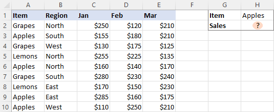
The question is - how do you get a total of sales for a certain item?
The first idea that comes to mind is using a SUMIF formula in its pure form:
=SUMIF(A2:A10, "apples", C2:E10)
Unfortunately, this won't work. The reason is that the dimensions of sum_range are determined by Excel automatically based on the dimensions of the range argument. As our criteria range includes only one column (A2:A10), so does the sum range (C2:C10). The sum_range parameter defined in the formula (C2:E10) actually determines only the upper left cell of the range that will be summed. As a result, the above formula will add up the apples sales only in column C. Not what we are looking for, eh?
The simplest working solution that suggests itself is to create a helper column summing the numbers for each individual row, and then use that column for sum_range.
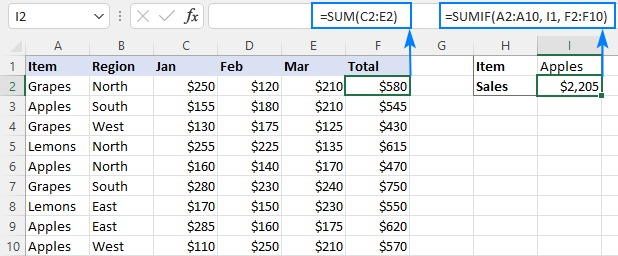
So, go ahead and place a SUM formula in F2, then drag it down across as many cells as needed:
=SUM(C2:E2)
After that, you can quickly have the job done:
=SUMIF(A2:A10, I1, F2:F10)
Where I1 is the item of interest.
In the above formula, sum_range is of the same size as range (1 column and 9 rows), so it works without a hitch:
If the layout of your worksheet does not have room for any extra columns, then apply one of the following solutions.
SUMIF multiple columns
The idea is to write a separate SUMIF formula for each of the columns you want to sum, and then add up the results:
Or
A practical implementation looks as follows:
=SUM(SUMIF(A2:A10,H1,C2:C10), SUMIF(A2:A10,H1,D2:D10), SUMIF(A2:A10,H1,E2:E10))
Or
=SUMIF(A2:A10, H1, C2:C10) + SUMIF(A2:A10, H1, D2:D10) + SUMIF(A2:A10, H1, E2:E10)
You can also "hardcode" the condition in the formula if needed:
=SUMIF(A2:A10, "Apples", C2:C10) + SUMIF(A2:A10, "Apples", D2:D10) + SUMIF(A2:A10, "Apples", E2:E10)

This works fine for a reasonable number of columns, but for a large dataset the formula becomes too long and difficult to read. In this case, the below solutions are more appropriate.
SUM as array formula
Another way to do a sum if in multiple columns based on one criterion is to construct an array formula:
For our sample dataset, the formula takes this form:
=SUM((C2:E10)*(--(A2:A10=H1)))
Or
=SUM((C2:E10)*(--(A2:A10="Apples")))
In Excel 2019 and older, you should press Ctrl + Shift + Enter to complete the formula correctly. In Excel 365 and Excel 2021, this works as a normal formula due to inbuilt support for dynamic arrays.
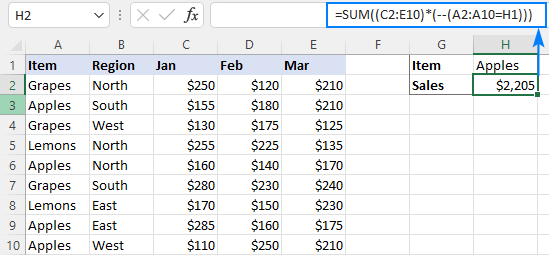
How this formula works:
The core concept is to multiply the elements of these two arrays:
- (C2:E10) - all the values in the sum range. In our case, the array contains 27 elements (3 columns and 9 rows: {250,120,210;155,180,210;130,175,125; …}
- (--(A2:A10=H1)) - compares each value in A2:A10 against the target item in H1. The result is an array of TRUE (the condition is met) and FALSE (the condition is not met) values, which is then converted into an array of 1's and 0's with the help of a double unary operator: {0;1;0;0;1;0;0;1;1}
Please pay attention that the first array is two-dimensional (each column of data is separated by a comma and each row by a semicolon) and the second one is a one-dimensional vertical array (1 column of data, rows are separated by semicolons). When the two arrays are multiplied, all the items of the 2D array in a given row are multiplied by the corresponding element of the 1D array:

As multiplying by zero gives zero, only the numbers for which the criterion is TRUE survive, and the SUM function adds them up:
=SUM({0,0,0;155,180,210;0,0,0;0,0,0;160,140,170;0,0,0;0,0,0;…})
To make the formula's logic easier to understand, you can write the first multiplier in this way:
=SUM((C2:C10 + D2:D10 + E2:E10) * (--(A2:A10=H1)))
This will produce an array of sums by row (like the helper column does in the very first example), which is then multiplied by an array of 1's and 0's:
{580;545;430;615;470;750;550;620;570}*{0;1;0;0;1;0;0;1;1}
The result of multiplication is served to SUM:
=SUM({0;545;0;0;470;0;0;620;570})
Don't like using arrays formulas in your sheet? Neither do I. Well, let's go check the next solution :)
SUMPRODUCT formula
The strategy described in the above example can also be implemented using the SUMPRODUCT function.
A real-life formula goes as follows:
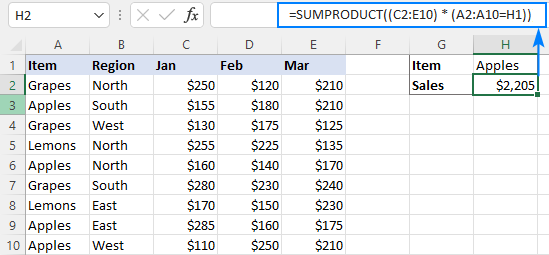
=SUMPRODUCT((C2:E10) * (A2:A10=H1))
The formula's logic is the same as in the previous example. The beauty of the SUMPRODUCT function is that it supports arrays natively, so it works nicely as a regular formula in all Excel versions.
Excel Sum If: multiple columns, multiple criteria
The three approaches we utilized to add up multiple columns with one criterion will also work for conditional sum with multiple criteria. The formulas will just become a little more complex.
SUMIFS + SUMIFS to sum multiple columns
To sum cells that match multiple criteria, you normally use the SUMIFS function. The problem is that, just like its single-criterion counterpart, SUMIFS doesn't support a multi-column sum range. To overcome this, we write a few SUMIFS, one per each column in the sum range:
Or
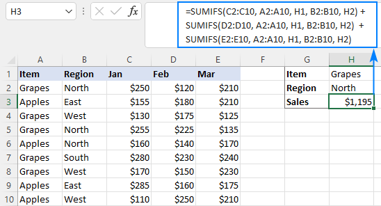
For example, to sum Grapes sales (H1) in the North region (H2), the formula is:
=SUMIFS(C2:C10, A2:A10, H1, B2:B10, H2) + SUMIFS(D2:D10, A2:A10, H1, B2:B10, H2) + SUMIFS(E2:E10, A2:A10, H1, B2:B10, H2)
Array formula to conditionally sum multiple columns
The SUM formula for multiple criteria is very much like that for a single criterion - you just include additional criteria_range=criteria pair(s):
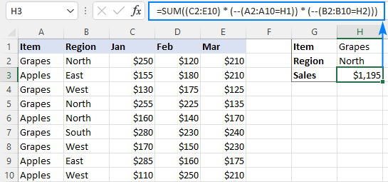
For instance, to sum sales for the item in H1 and the region in H2, the formula goes as follows:
=SUM((C2:E10) * (--(A2:A10=H1)) * (--(B2:B10=H2)))
In Excel 2019 and older, remember to press Ctrl + Shift + Enter to make it an CSE array formula. In dynamic array Excel 365 and 2021, a normal formula will work fine as shown in the screenshot:
SUMPRODUCT formula with multiple criteria
The easiest way to sum multiple columns based on multiple criteria is the SUMPRODUCT formula:
As you can see, it's very similar to the SUM formula, but does not require any extra manipulations with arrays.
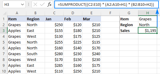
To sum multiple columns with two criteria, the formula is:
=SUMPRODUCT((C2:E10) * (A2:A10=H1) * (B2:B10=H2))
These are the 3 ways to sum multiple columns based on one or more conditions in Excel. I thank you for reading and hope to see you on our blog next week!
Practice workbook for download
Sum if multiple columns - examples (.xlsx file)
 by
by
93 comments
hi
i need to get the summary of training hours for a certain employee in a year. 1st column is name of employees, 2nd column onwards is the hours rendered per type of training which is indicated at the top most row. One training can have multiple occurrence for the year. The summary and record are in a separate sheet. Hope you can help me with this. thank you in advance
Hi! Based on your description, it is hard to completely understand your task. However, I’ll try to guess and offer you the following SUMPRODUCT formula:
=SUMPRODUCT((A2:A10="Name")*B2:E10)
If an employee's name is repeated more than once in a column, this formula will calculate the sum of the numbers in all columns B:E for that employee. If this is not what you wanted, please describe the problem in more detail.
column A customer name
Column B, row 1 onwards month eg: Jan, Feb....etc
Column B row 2 onwards different product eg: Apple, grapes.
what is the suggest formula can use to sum total quantity for each coustomer in column A from Jan (to mar (based quarterly order) to forecast the trend?
Hi! There is no quantity you want to summarize in your data description. However, I’ll try to guess and offer you the following formula:
=SUMPRODUCT((A3:A11="A") * ((B3:F11) * (B2:F2="Apple") * ((B1:F1="Jan") + (B1:F1="Feb") + (B1:F1="Mar"))))
I recommend reading this guide: Excel SUMPRODUCT function with formula examples.
Hi Alexander
Thanks for suggestion.
I would like to sum total quantity of each month for each type product of each customer. As there will be has 12 months in row and 20 products for multiple customer. So would like to know sum order for each type product in each month of every customer.
Hi! In your first question, you wanted to summarize January through March. Leave only one month in the formula if you only want the amount for one month. If this formula does not work for you, please explain in detail why.
=SUMPRODUCT((A3:A11="A")*((B3:F11)*(B2:F2="Apple")*(B1:F1="Jan")))
Hi,
I have a problem sum values using SUMIFS in my sheet. This sheet look like this:
Column1=name of companies
column2=Date payment received (Jan)
Column3=payment value
Column4=Date payment received (Feb)
Column3=payment value .......
all until December
I want to sum (payment values) with dates from-to for each company.
I appreciate any assistance on this matter.
Thanks
Arnold
Hello Arnold!
All the necessary information is in the article above. Here is a sample formula for the first two months. You can read more about how the SUMIFS function works with dates by clicking here: Using Excel SUMIFS with dates.
=SUMIFS(C2:C10,A2:A10,L1,B2:B10,">"&K1,B2:B10,"<"&K2) + SUMIFS(E2:E10,A2:A10,L1,D2:D10,">"&K1,D2:D10,"<"&K2)
Hi,
Can you please guide me with?
i have two sheets 1st is Monthly and amount and 2nd is Platform and amount.
now i have to make summery in that summery.
what formula will i use that amount will automaticly change.
Hi! Unfortunately, this information is not enough to give you any advice. Please provide me with an example of the source data and the expected result.
Just wanted to say Thanks Alex, this sumproduct formula will save me time as the sumifs was not playing nice.
In your example 'Array formula to conditionally sum multiple columns':
=SUM((C2:E10) * (--(A2:A10=H1)) * (--(B2:B10=H2)))
If your column A had many types of fruit and you wanted to return the total sales value of say {"Apples","Grapes","Pears"} over the 3 months irrespective of Region, how would you include this, preferably in the syntax you have used in this example?
I would also like to replace the Month names for dates e.g. 01/03/2024 which I can then format as MMM-YY, so that I can then also add a filter (--(C1:N1<=Q1), where Q1 is the month I select from a drop down list - so that I can pick up 12 months worth of year-to-date values of whichever combinations of product in column A that I want, for whichever month I want.
Can I achieve both filters in the one formula using the SUM array syntax?
Hello! To use multiple criteria in column A, the formula might look something like this:
=SUMPRODUCT((C2:E10) * ((A2:A10=H1)+(A2:A10=I1)+(A2:A10=J1)) * (--(B2:B10=H2)))
Look for the example formulas here: Excel SUMPRODUCT function with formula examples.
Also note that formatting the date as MMM-YY does not change the date value in the cell. Try to use the recommendations described in this article: Excel IF between two dates.
I hope it’ll be helpful. If something is still unclear, please feel free to ask.
Thanks very much, that does help, shortens my formulae a bit and allows me to bring the date <= criteria in too.
However I was hoping there would be an even more concise way to write this part
((A2:A10=H1)+(A2:A10=I1)+(A2:A10=J1))
as I am referencing an external workbook and 11 or 12 different items (e.g.. fruit as in your example), so having to replicate the A2:A10= part 12 times over with a long file path & filename each time still makes the formula hard to read. Is there any other way to write this? Thankyou.
I'm really sorry, we cannot help you with this.
Hi, Alexander. Thanks for sharing this formula. Using your formula, I managed to get the exact sum of the value according to the criteria set forth. However, in order to make sense of the dynamic nature of the data, could you please help recommend me a formula that could:
1. Expand my columns dynamically to include larger size sample (according to my input), ie. from C13:P33 to C13:HO33. The values from Q33 to HO33 based on current sample are simply zero "0" OR
2. Ignore the column headers (referring to my data set below re characterized as "Group X") are meanwhile indicated as "#N/A" if not
Currently, my data looks to be:
Unit Unit 1 Unit 2 Unit 3 Unit 4 Unit 5
Group Group 1 Group 1 Group 2 Group 3 Group 3
Unit # 1 2 3 4 5
Column # 2 3 4 5 6
Speed Code Value Value Value Value Value
ABC 282735.9788 282735.9788 282735.9788 282735.9788 282735.9788
DEF 6274.64382 6274.64382 6274.64382 6274.64382 6274.64382
GHI 0 0 0 0 0
JKL 500 500 500 500 500
LMN 16203.75 23816.25 16203.75 16203.75 16203.75
The formula that worked so far is =SUM((Booking!$C$13:$P$33)*(--(Booking!$B$13:$B$33=M$12))*(--(Booking!$C$5:$P$5=$AD14))).
M12=Speed Code criteria while AD14=Group criteria.
For the 1st option, I've tried VLOOKUP & HLOOKUP to indicate a dynamic column range but these 2 didn't work.
While for the 2nd option, I've tried incorporating SUMIF as subset of SUM, alas - it didn't work as well.
Really hoping you could help me solve this issue as I've been working on this for a week already.
Thanks a lot!
Hi! If I understand your problem correctly, you can use dynamic named range. The following tutorial should help: How to create and use dynamic named range in Excel. You can also convert your range to an Excel table so your formulas automatically use the new data. You can also find useful information in this article: Structured references in Excel tables.
I hope it’ll be helpful.
had similar issue where my data was spread across multiple columns, but I only wanted to sum based on BOTH row & column criteria. The row criteria was a "single" row, so I was able to use INDIRECT combined w/MATCH to determine which row to add, then basic SUMIFS for my column criteria.
My data has item # down 1st column and weekly buckets across the top. I need to add all values w/in a month for a 'selected' item.
SUMIFS(INDIRECT("Export!"&MATCH($A2,Export!$A:$A,0)&":"&MATCH($A2,Export!$A:$A,0)),Export!$1:$1,">="&'Open and Planned'!C$1,Export!$1:$1,", =, <.
Does anyone have another/easier way to achieve the same?
Hi! It is very difficult to understand a formula that contains unique references to your workbook worksheets. Additionally, the formula has been incompletely written.
looks like part of my message cut off. my formula is SUMIFS(INDIRECT("export!"&MATCH($A2,Export!$A:$A,0)&":"&MATCH($A2,Export!$A:$A,0)),Export!$1:$1,">="&'Open and Planned'!C$1,Export!$1:$1,"<"&'Open and Planned'!D$1)
where Export is the worksheet name that contains the sum range, cell A2 is the item #, cells C1/D1 are the start/end dates to check
Can/how would you SUM multiple workbooks linked together that have a SUMIF formula? Basically trying to sum 29 workbooks with a SUMIF column with 1 condition.
Your explanation is not very clear, but perhaps you will find the Consolidate Sheets tool useful. It can summarize data from multiple worksheets. The tool is included in the Ultimate Suite for Excel and can be used in a free trial to see how it works.
Hi Alexander, how can I replace the '=' in criteria with to indicate a range - my formula returns #VALUE!
Sample of my formula shown below
=SUM((D:O)*(--(B:B>1099))*(--(B:B<1200))*(--(C:C<Last_FY)))
Thanks in advance
Nanette
Hi! Your formula is error free and should work. The error occurs as a result of your data, which I can't see and can't verify.
Hi Alexander, I am so grateful
your response encouraged me to keep testing my formulas against my data. I thought the problem was with using greater-than and less-than signs. What I found was that I was 1) needing to exclude my headings from my ranges of numbers; 2) Ctrl, Shift & Enter to enter my formula over an array.
Formulas that were 25 + lines long are now around 5 lines with correct outputs. One of my corrected formulas is shown below -
{=SUM(('CF InData'!$D2:$O5000)*(--('CF InData'!$B2:$B5000>=1100))*(--('CF InData'!$B2:$B5000<=1199))*(--('CF InData'!$C2:$C5000=1100","<=1199"},'CF InData'!$C:$C,"="&Last_FY))*1}
Thank you so sincerely :)
Hi Alexander
My formula did not copy well with bits being ignored between the greater than and less than signs again. You can delete my reply above, but I really did wish to thank you publicly.
Kind regards
Nanette
Hi I want to get sum
all data in same row with different columns
the criteria is lookup specific name & get sum of third column in same row
please keep in mind all data in same row but multiple columns
pleas share solution if any?
Hi! Unfortunately, this information is not enough to recommend a formula to you. To understand what you want to do, give an example of the source data and the expected result.
See my comment for the 'solution' I used which may work for you - a combination of INDIRECT & MATCH to obtain the row # for the sum range, then normal SUMIFS criteria to get the right column(s).
My data has item # down 1st column and weekly buckets across the top. I need to add all values w/in a month for a 'selected' item.
SUMIFS(INDIRECT("export!"&MATCH($A2,Export!$A:$A,0)&":"&MATCH($A2,Export!$A:$A,0)),Export!$1:$1,">="&'Open and Planned'!C$1,Export!$1:$1,"<"&'Open and Planned'!D$1)
where Export is the worksheet name that contains the sum range, cell A2 is the item #, cells C1/D1 are the start/end dates to check. Therefore, the SUMRANGE is the "row" on Export tab that matches the item #.
I don't know if this is the "right" way to go about this, but it works ;-)
This was so helpful! Thank you for explaining the different options in a way that is so comprehensive and easy to follow.
Hi
Column1 Prod a Prod B Prod C Prod D Prod E Prod F
January 1
January 1
January 1
January 1
February 1
February 0.5
March 1
How do I summarise the total for each product by month in the following table?
Jan Feb Mar Apr May Jun
Prod A
Prod B
Prod C
Prod D
Prod E
Prod F
Hi! For your data, you must use a separate formula for each sum. For example, product A for January:
=SUMIFS(B2:B100,A2:A100,"January")
Hai, i have a question, if i want to sum item,between month from januari to februari or from januari to march or only on januari, with the help of data validation so its change conditionally if i select certain month or the last three month. Please Help, Thank you.
Hello! I’m sorry, but your description doesn’t give me a complete understanding of your task. Maybe this guide will be helpful: SUMIF with dates.
Item code = column A
qty ordered = Column B
Needing to find a formula to look at item code in column A, and the qtys in column B and total together all qtys for specific item code on a separate sheet.
Please help I have tried (almost) everything. The data will be filled in over time, not all at once, so I need something ongoing.
Hi! You can see an example of the sum formula for item code in the second paragraph of this article: How to use SUMIF function in Excel. You can also find useful information in this article: Excel reference to another sheet or workbook (external reference). I hope my advice will help you solve your task.
I have a table containing sales unit data per month ( in each column) and a different column containing retail value of each SKU, I am trying to create a summary by category using sumproduct and sumifs but it gives me value error.
this is the formula i am using,
=SUMPRODUCT((G5:G34=N5)*(I4:K4=O4),H5:H34,I5:K34)
Here is the sample data table
Item# Des Cat SRP Jan Feb March
10122 NARS RCC CAFE CON LECHE RADIANT CREAMY CONCEALER 42 1 2 3
122610 NARS RCC MARRON GLACE RADIANT CREAMY CONCEALER 42 4 5 6
122710 NARS RCC TIRAMISU RADIANT CREAMY CONCEALER 42 7 8 9
12281 NARS RCC SUCRE D'ORGE RADIANT CREAMY CONCEALER 42 10 11 12
12291 NARS RCC WALNUT RADIANT CREAMY CONCEALER 42 13 14 15
Hi! You cannot multiply the values of arrays that have different sizes. (G5:G34=N5)*(I4:K4=O4) - impossible.
Hi,
I am trying to pull data from one tab to another, based on 2 descriptions. So the descriptions in 2 cells on Tab 1 e.g. E10:E64 and F10:F64 dictate if a figure (£) from a range of cells, say D1-D20 is copied into another cell, on another tab.
It works currently if one description dictates the data which is pulled across, using formula - SUMIF('Tab2'!E$10:E$64,B12,'Tab2'!I$10:I$63)
But I want both Criteria to be met, before the data is pulled across.
Any help is appreciated!
Hi! If you want to find an amount by two criteria, try using the SUMIFS function.
I am trying above formula where data is in one sheet and the formula in other sheet (same workbook) but its not working? while i tried same formula but in same sheet it worked. Is there restriction for using the formula in different sheet than the data sheet?
Hi! There are no such restrictions. I recommend that you read these recommendations: How to SUMIF between two sheets. I hope it’ll be helpful.
Hello!
The SUMIF function works fine between the sheets & I have no issue with that. What i was trying to use the sum array / sumproduct as explained above, but I was getting error. I made some research & found that the error is due to the header (containing alphabet characters) in Value column. It works only when the value column content are numbers only.
Thanks Alexander!
thank you so much for the detailed explanation!
may i ask if this is applicable to summing multiple rows with a single criteria?
How can i match 2 criteria and give result.
example:
Sheet 1
A1 = item code
B1= Location (4 different location)
result=?
Sheet2 is data sheet
A:A= item code
B:B=locations
C:C= value
so if a1 and b1 matches with a:a and b:b then total to be resut.
Hi! If I understand you correctly, to summarize values by multiple criteria, use the SUMIFS function. For more information, please visit: How to use Excel SUMIFS and SUMIF with multiple criteria. I hope it’ll be helpful. If something is still unclear, please feel free to ask.