Every once in a while each Google Sheets user faces the inevitable: combining several sheets into one. Copy-pasting is tedious and time-consuming, so there has to be another way. And you're right — there are several ways, in fact. So get your tables ready and follow the steps from this article.
All the ways I describe can be used to process large tables. But to keep this guide as clear as possible, I'll keep my tables short and am going to cut down to a couple of sheets.
Reference cells in Google Sheets to pull data from another tab
The easiest way comes first. You can pull entire tables to one file by referencing cells with data from other sheets.
Note. This will do if you need to merge two or more sheets within one Google spreadsheet. To merge multiple Google spreadsheets (files) into one, jump right to the next method.
So, my data is scattered all over different sheets: June, July, August. I'd like to pull data from July and August into June to have one table as a result:
- Find the first blank cell right after your table (the June sheet for me) and place the cursor there.
- Enter your first cell reference. The first table I want to retrieve starts from A2 in the July sheet. So I put:
=July!A2Note. If there are spaces in your sheet name, you must wrap it in single quotes like this:
='July 2022'!A2This immediately replicates whatever lies in that cell:

Note. Use relative cell reference so it changes itself when copied to other cells. Otherwise, it will return incorrect data.
- Make sure the cell with the reference is selected and click on that little blue square at its bottom right corner. The mouse cursor will turn into a big black plus sign. Keep the mouse pressed and drag the cursor to as many columns to the right as you need to fill them with new records:

- Select this entire new row, click that little blue square once again, hold and drag your mouse down — this time to fill entire rows with cell references and bring new data from another sheet:

Though this is probably the first way you may think of to pull data from another tab, it's not the most elegant and quick. Luckily, Google prepared other instruments specially for this purpose.
Copy the tabs into one spreadsheet
One of the standard ways is to copy the tabs of interest into the destination spreadsheet:
- Open the file that contains the sheet(s) you want to transfer.
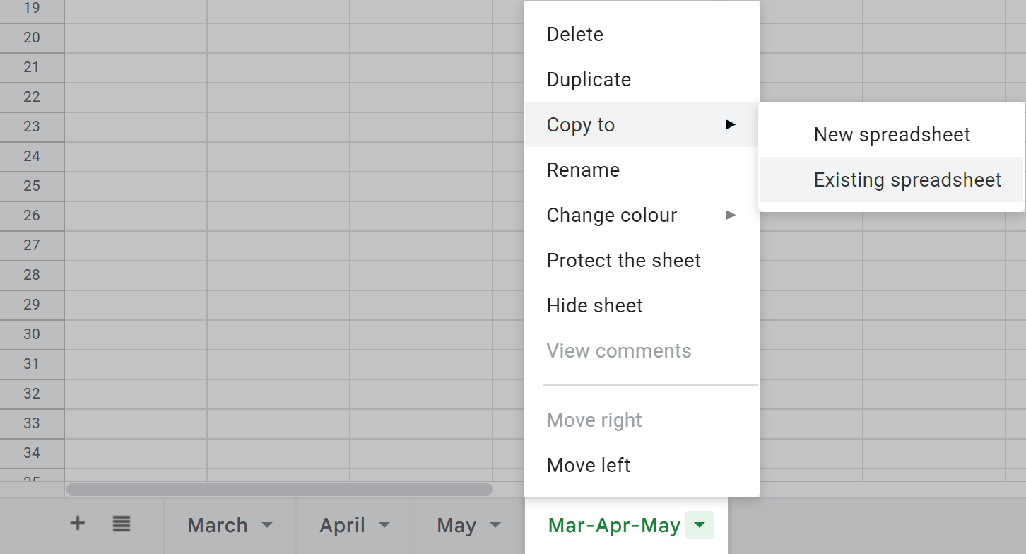
- Right-click the first tab you need to export and choose Copy to > Existing spreadsheet:
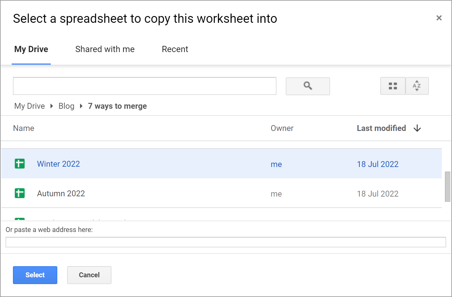
- The next thing you'll see is the pop-up window inviting you to select the spreadsheet. Browse for it, click on it to highlight it, and press Select when you're ready:
- Once the sheet is copied, you'll get a corresponding confirmation message:

- You can either hit OK and continue with the current sheet or follow the link called Open spreadsheet. It will instantly get you to another spreadsheet with the first sheet already there:

Export/import sheets
Another way to import data from multiple Google Sheets is to export each sheet first, and then import them all to a necessary file:
- Open the spreadsheet that contains the sheet you'd like to pull the data from.
- Make the sheet of interest active by selecting it.
- Go to File > Download > Comma-separated values (.csv):

The file will be downloaded to your computer.
- Then open another spreadsheet — the one you'd like to add the sheet to.
- This time, pick File > Import from the menu and go to the Upload tab in the Import file window:
- Hit Select a file from your device and find the sheet you've downloaded just now.
- Once the file is uploaded, you'll see a window with additional options for importing the sheet. To add the contents of that another sheet after your existing table, pick Append to current sheet:

Tip. Among other settings, feel free to specify the separator and convert text to numbers, dates, and formulas.
- As a result, you'll get two sheets merged — one table under another:

But since it is a .csv file you need to import, the second table remains formatted in a standard way. You will have to spend some time formatting it as you need.

Google Sheets functions to combine data from multiple spreadsheets
Of course, it wouldn't be Google if it didn't have functions to merge data in Google Sheets.
IMPORTRANGE to import data from multiple Google sheets
As the name of the function suggests, IMPORTRANGE imports data from multiple Google spreadsheets into one sheet.
Tip. The function helps Google Sheets pull data from another document as well as from other tabs from the same file.
Here's what the function requires:
- spreadsheet_url is nothing else than the link to the spreadsheet from where you need to pull the data. It must always be put between double-quotes.
- range_string stands for those cells specifically that you need to bring to your current sheet.
And here's the pattern I follow to import data from multiple Google Sheets using IMPORTRANGE:
- Open the spreadsheet from which you want to pull the data.
Note. Make sure you have at least viewing access to that file.
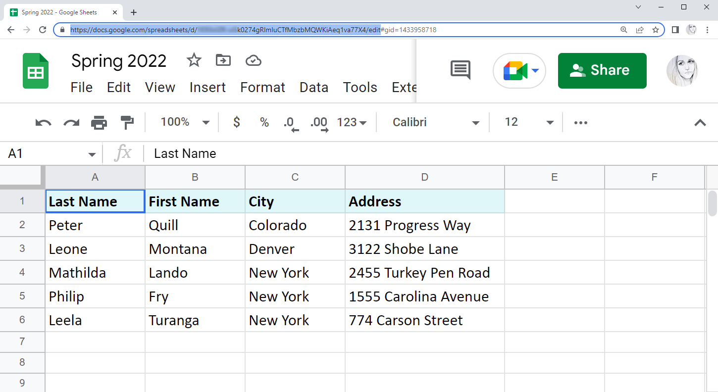
- Click the browser URL bar and copy the link to this file right till the hash sign (#):
- Return to the spreadsheet where you want to add the info to, enter the IMPORTRANGE to where the borrowed table should appear, and insert the link as the first argument. Then separate it from the next part with a comma:
- For the second part of the formula, type in the name of the sheet and the exact range that you want to pull. Confirm by pressing Enter.
Note. Wrap the second argument in double quotes as well:
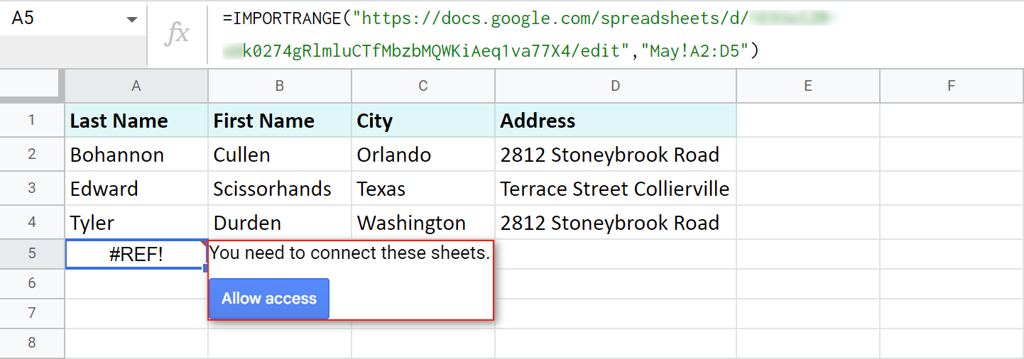
=IMPORTRANGE("https://docs.google.com/spreadsheets/d/XYZk0274gRlmluCTfMbzbMQWKiAeq1va77X4/edit","May!A2:D5") - Though the formula looks ready now, it will return the #REF error from the start. That's because the first time you try to pull data from some spreadsheet, IMPORTRANGE will ask for access to it. Once the permission is granted, you will easily import records from other sheets of that file.
Click the cell with the error and press that blue Allow access prompt:
- Once the formula connects to that other sheet, it will import data from there:
Note. You'll need this URL even if you're going to combine sheets from the same file.
Tip. Though Google says the function requires the whole URL, you can easily get by with a key — a part of the URL between /d/ and /edit:
...google.com/spreadsheets/d/XYZk0274gRlmluCTfMbzbMQWKiAeq1va77X4/edit

Note. Remember, the link should be surrounded by double quotes.
Note. By allowing access, you let the Sheets know you don't mind any existing or potential collaborators on this spreadsheet accessing data from another file.
Note. IMPORTRANGE doesn't pull the formatting of the cells, only values. You will need to apply formatting manually afterwards.
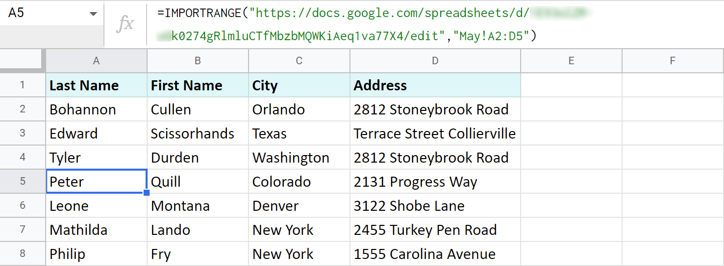
Tip. If the tables are rather big, just allow some time for the formula to pull all records.
Note. The records returned by the function will be updated automatically if you change them in the original file.
Google Sheets QUERY to import ranges from multiple sheets
And thus, without haste, we've come to the QUERY function once again. :) It is so versatile that can be used in Google spreadsheets to combine data from multiple sheets (within the same file) as well.
So, I want to merge three different Google sheets (from one file): Winter 2022, Spring 2022, and Summer 2022. They contain the names of all employees who became best in their jobs in different months.
I go to the first sheet — Winter 2022 — and add my QUERY right under the existing table:
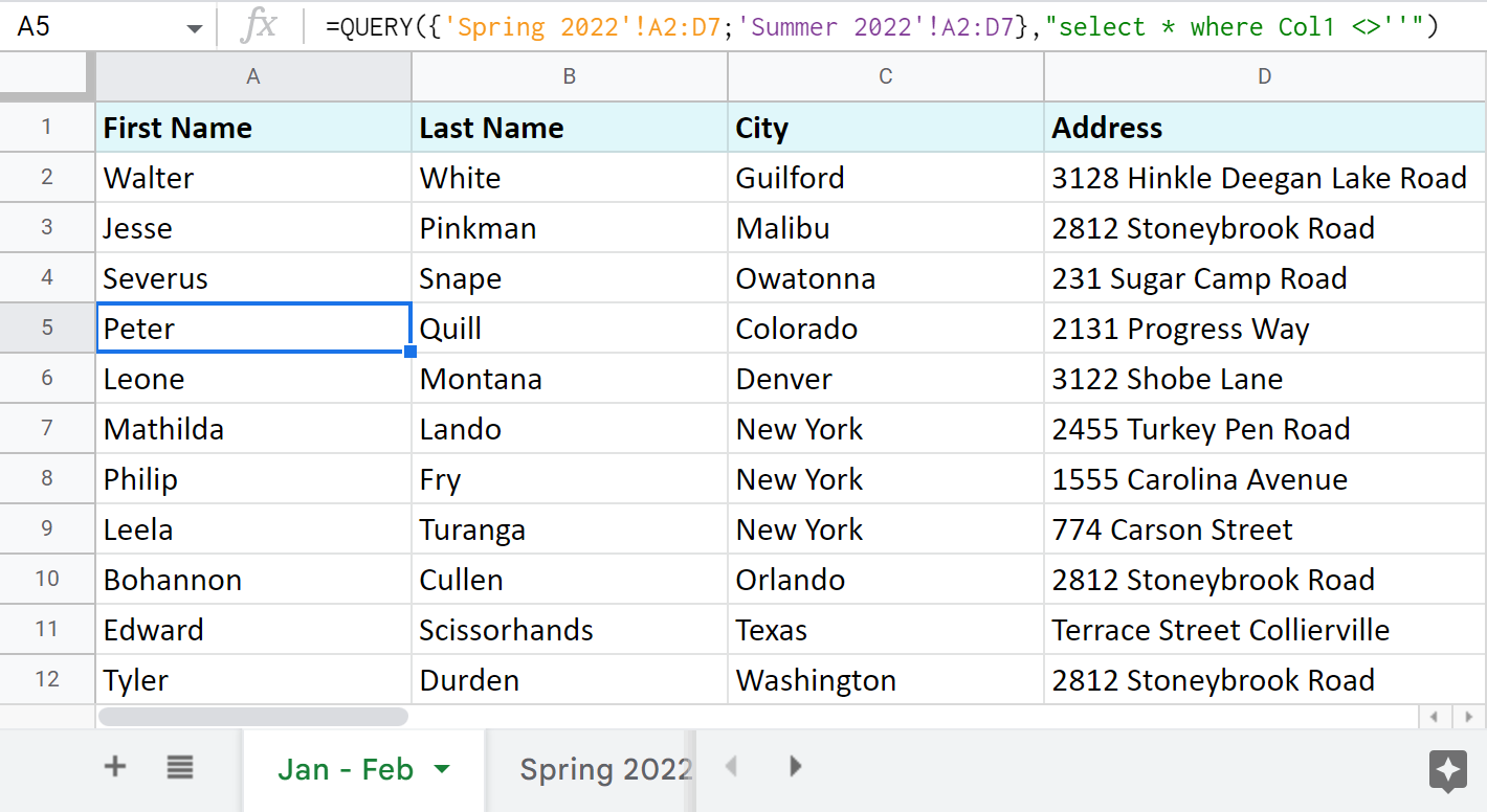
=QUERY({'Spring 2022'!A2:D7;'Summer 2022'!A2:D7},"select * where Col1 <>''")
Let's see what it all means:
- {'Spring 2022'!A2:D7;'Summer 2022'!A2:D7} — are all the sheets and ranges I need to import.
Note. The sheets should be written in between the curly brackets. If their names contain spaces, use single quotes to list the names.
Tip. Separate the ranges with a semicolon to pull data from different tabs one under another. Use commas instead to have them imported side by side.
Tip. Feel free to use such infinite ranges as A2:D.
- select * where Col1 <>'' — I tell the formula to import all records (select *) only if cells in the first column of the tables (where Col1) are not blank (<>''). I use a pair of single quotes to indicate the non-blanks.
Note. I use <>'' because my column contains text. If your column contains other data type (e.g. date or time, etc.), you need to use is not null instead: "select * where Col1 is not null"
As a result, two tables from other sheets have been consolidated into one sheet one under another:
Tip. If you'd like to use Google Sheets QUERY to import ranges from multiple separate spreadsheets (files), you will have to implement IMPORTRANGE. Here's a formula to pull your data from other documents:
=QUERY({IMPORTRANGE("XYZk0274gRlmluCTfMbzbMQWKiAeq1va77X4","Mar-Apr-May!A2:D6");IMPORTRANGE("XYZahJZHSlhMGLSW_xA6ZBqNmt1I0ADo4N4M","Jun-Jul-Aug!A2:D4")},"select * where Col1<>''")
Tip. I use the keys from URLs rather than entire links in this long-enough formula. If you're not sure what that is, please read here.
Tip. You can also use QUERY to merge two Google sheets, update cells, add related columns & non-matching rows. Check this out in this blog post.
3 quickest ways to merge multiple Google sheets
If standard ways of Google spreadsheets to combine data from multiple sheets seem dull, and the functions scare you off, there's an easier approach.
Combine Sheets add-on
This first special add-on — Combine Sheets — was designed with a single purpose: import data from multiple Google sheets.
Add it to your Google Sheets
It's clever enough to recognize the same columns in different sheets and bring data together accordingly if you need.

All you are to do is:
- Select sheets or entire spreadsheets to merge and specify the ranges if necessary. A quick search across your Drive makes this even faster.
- Choose how to pull the data:
- as a formula. Mark the checkbox called Use a formula to combine sheets if you want to have a master sheet that will dynamically change based on your original contents.
Although you won't be able to edit the resulting table, its formula will be always linked to the source sheets: edit a cell or add/remove entire rows there, and the master sheet will be altered accordingly.
- as values. If editing the resulting table manually is more important, ignore the above option and all data will be combined as values.
Extra options are here for fine-tuning:
- join records from the same columns into one column
- keep the formatting
- add a blank line between different ranges to notice them right away
- as a formula. Mark the checkbox called Use a formula to combine sheets if you want to have a master sheet that will dynamically change based on your original contents.
- Decide where to place the merged table: new spreadsheet, new sheet, or in a location of your choice.
Here's a quick demonstration of how I combined my three small tables with the add-on:
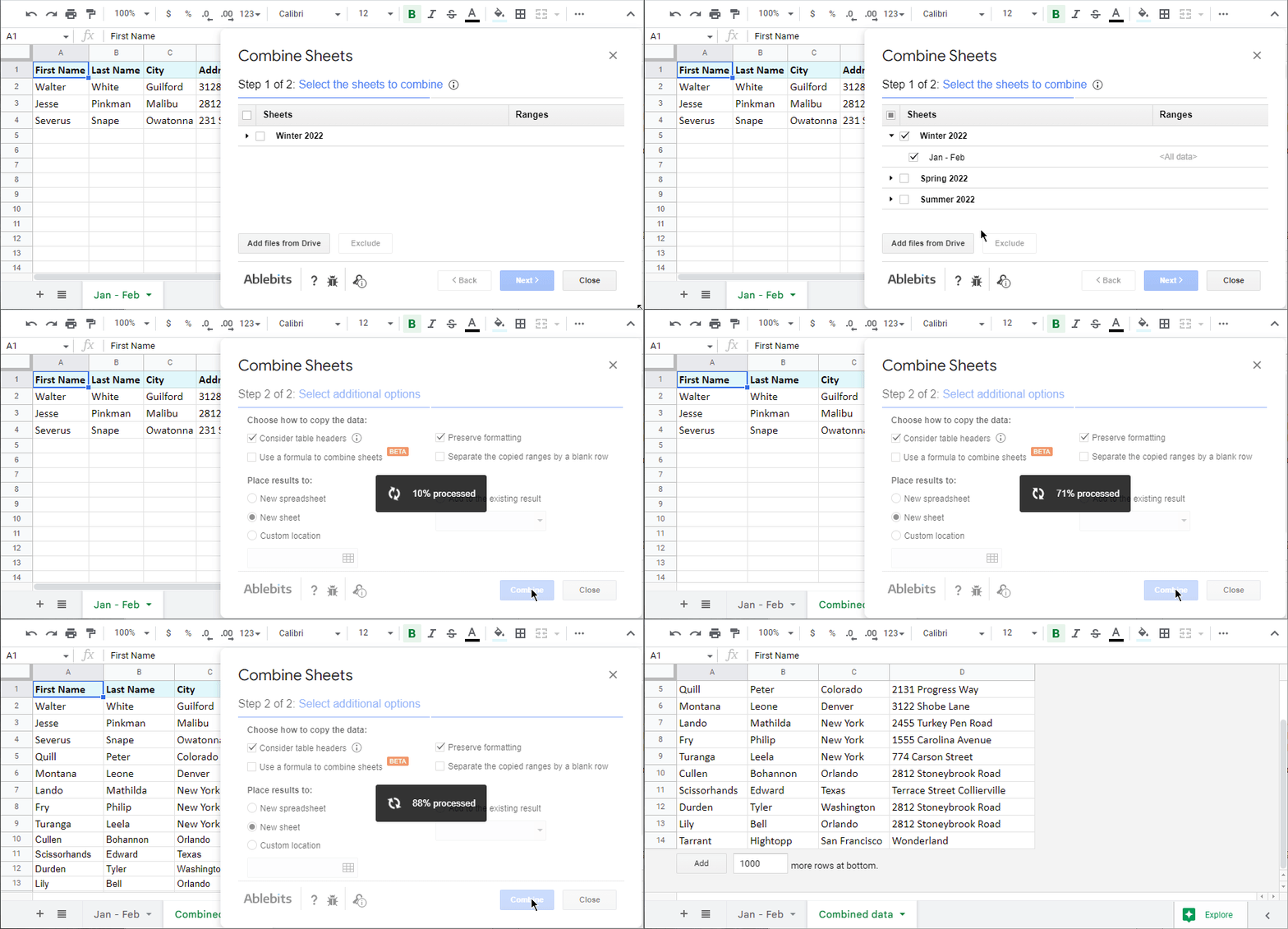
Of course, your tables can be much bigger and you can merge lots of different sheets as long as the resulting file doesn't exceed the 10M cell-limit.
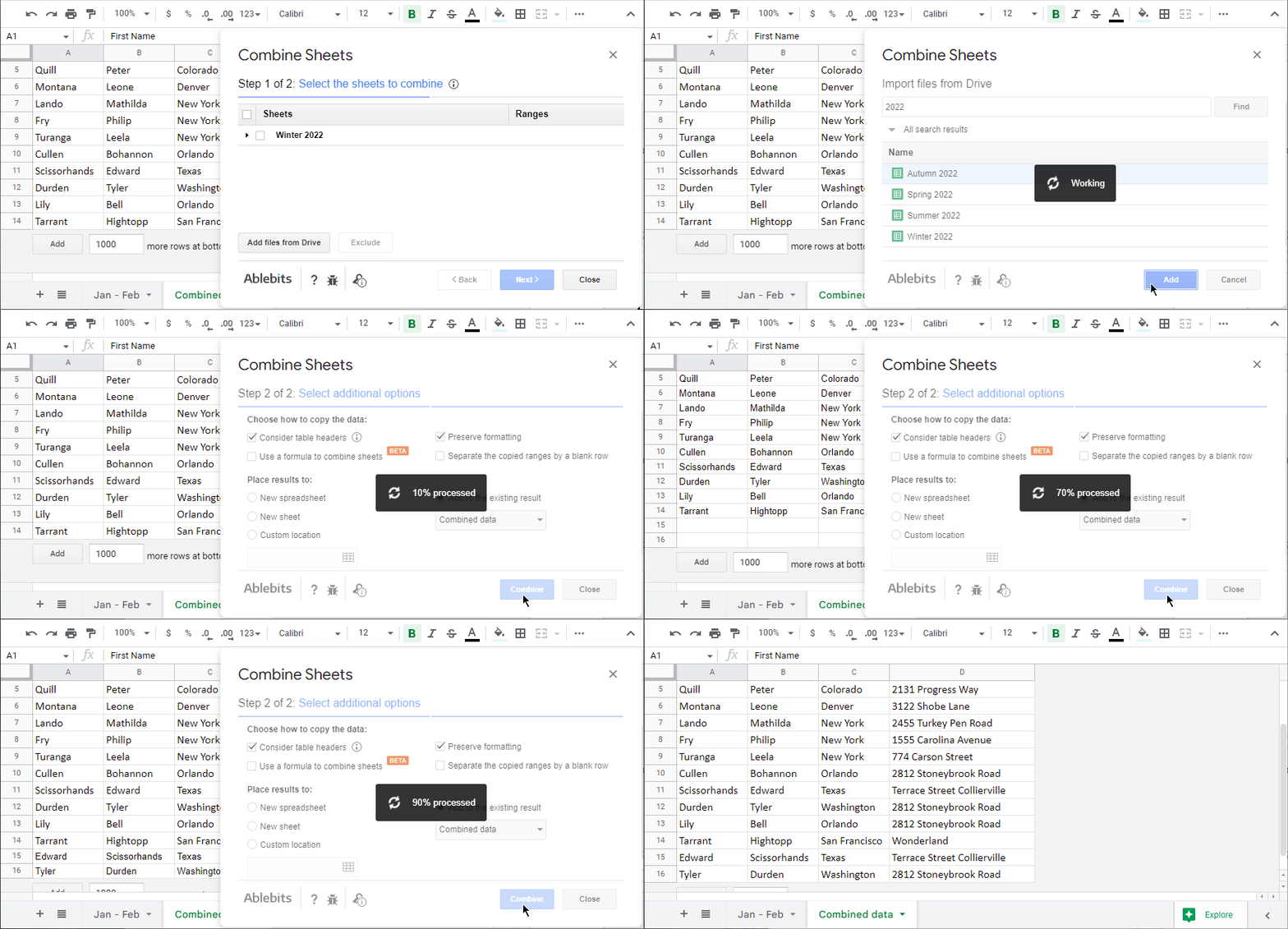
One of the options this add-on offers is to add more sheets to your previously combined data. In this case on step 1, you need to pick not only the data to combine but also the existing result. Here's how it looks:
Video: How to combine multiple Google sheets into one
Check out the help page for Combine Sheets or watch this 3,5-minute tutorial:
Consolidate Sheets add-on
Consolidate Sheets is another handy tool among our add-ons. Its main difference from the aforementioned tool is the ability to add up data in columns in Google Sheets (or rows, or single cells, for that matter).
Add it to your Google Sheets
Consolidate Sheets also recognizes common headers in all the Google sheets to join, even if they are in the leftmost column and/or the first row. There's always an option to merge Google sheets and calculate cells based on their place in the tables.
Let me break it down into steps for you as well:
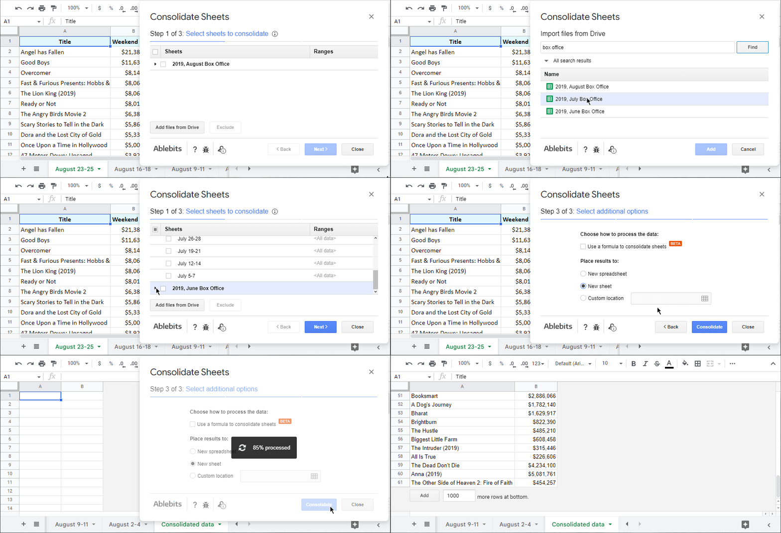
- Select sheets to consolidate. Import more files from Drive if necessary straight from the add-on.
- Pick the function to consolidate in Google Sheets.
- Choose the way to add up cells in Google Sheets: by labels (header labels, left column labels, or both) or position.
- Decide where to place the consolidated data: new spreadsheet, new sheet, or any specific location within the opened file.
Here's how this process looks:
There's also an option to consolidate all your sheets using a formula. This way your result will change in sync with the values in the source sheets:
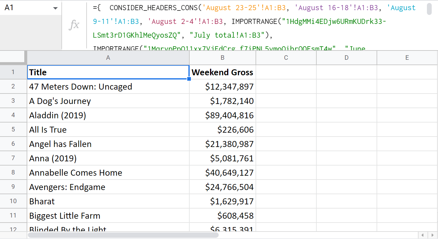
Note. There are some peculiarities you need to know about how the formula works. For example, if you consolidate from multiple different files, there will be an extra step to connect the sheets for the IMPORTRANGE in use. Please visit the instructional page for Consolidate Sheets for these and other details.
Video: How to consolidate multiple Google sheets into one
Here's a 4-minute demo-video about the add-on work:
I truly encourage you try this add-on.
Add it to your Google Sheets
You'll see for yourself how much extra time you'll have after incorporating this tool to your daily work.
Merge Sheets add-on
There's one more add-on worth mentioning — Merge Sheets. It matches records from the same column in several tabs/files and then pulls related data from the lookup tabs/files into the main one. Hence, you always have an up-to-date spreadsheet at hand.
Add it to your Google Sheets
There are 5 straightforward steps:
- Select your main sheet.
- Select your lookup sheet (even if it's in another spreadsheet).
- Choose columns where matching records may occur.
- Tick of the columns with records to update.
- Tweak any additional options that will help you merge two sheets and achieve the best result possible.
You can even save the settings into reusable scenarios and run them later in a click.
Video: How to merge Google sheets
I know a picture is worth a thousand words, so here's a 3-minute video tutorial on Merge Sheets for you:
Ready to try Merge Sheets for yourself?
Add it to your Google Sheets
Or visit this help page for details about each step and setting.
On this note, I'm going to finish this article. Hope these ways of pulling data from multiple different sheets into one will be of use. As always, looking forward to your comments!
 by
by
234 comments
This guide is incredibly helpful for anyone looking to streamline their Google Sheets workflow! Merging multiple sheets without the hassle of copy-pasting can save so much time. I especially appreciate the detailed instructions on using functions like IMPORTRANGE and QUERY. Thanks for sharing these practical tips!
This guide on merging Google Sheets without copy-pasting is a game-changer! The methods like IMPORTRANGE and using add-ons streamline the process and save so much time. Natalia's clear instructions make it easy to follow along, ensuring users can efficiently combine their data. A must-read for any Google Sheets user!
Great article, Natalia! Merging Google Sheets without copy-pasting is such a game changer. I love how you break down methods like IMPORTRANGE and QUERY; these functions truly allow users to delve into their data efficiently. Your tips on using add-ons are also valuable for those seeking the ultimate convenience. Thanks for sharing!
Thank you! I'm happy to know you've found the article useful :)
Great guide on merging Google Sheets without tedious copy-pasting! The methods you outlined—using cell references, combining tabs, exporting/importing sheets, and leveraging functions like IMPORTRANGE and QUERY—are incredibly useful. The add-ons for merging sheets are also a game-changer for efficiency. Thanks for sharing these practical solutions!
Appreciate your feedback!
Combining Google Sheets can be streamlined using methods beyond tedious copy-pasting. Utilize functions like IMPORTRANGE or QUERY for efficient data integration, or explore add-ons like Combine Sheets for a quicker solution. These techniques simplify merging large tables and save valuable time. Check out the article for step-by-step instructions!
I'm wondering if you might be able to help me out. I have about 20 different google sheets files - each user gets their own sheet to populate with information about their people. We need to consolidate the data from all of the sheets into a single sheet. I tried "combine sheets" but it didn't put the data in the right places. These are not different tabs, they're unique files.
Each sheet is formatted the same.
Each sheet has the same data fields (first name, last name, address, etc.), but the column header labels aren't at the top, the data starts at row 10.
Each sheet has a different number of records - anywhere from 5-120 per sheet
Any thoughts on how best to get the data into a single list? Thanks!!
Hello Sunshine,
Combine Sheets is perfect for the task even when your tables are in different files. You can select them all via the tool.
You can also specify the ranges, so having tables start from row 10 is also not a problem.
For us to be able to help you with the add-on, please email our support team directly (support@ablebits.com) with the screenshots of the following:
Our team will do their best to help. Thank you.
I actually tried again (and refined my ranges better) and it seems to be working! Thanks so much!!!
I think the issue was the I hadn't un-selected one of the sheets to extra data that I wasn't expecting was being pulled in. Great tool - will save me TONS of time!! Thanks for your help!
Thank you for your kind words, Sunshine. Great to hear the extension's working now! If you ever need assistance with it, feel free to reach out to our support team right away 😊
If it's not too much trouble for you, we would appreciate it if you rate our add-on and maybe write a few words on Google Workspace Marketplace. Your positive feedback motivates us to provide the best experience for you and helps others understand how our product makes their life easier 😊
Have a lovely week!
Hello!
I am trying to merge data from 6 different spreadsheets into one using the QUERY and IMPORTRANGE formula from above. I can get the formula to pull the data in for 1 spreadsheet at a time, but I receive an error when I try multiple spreadsheets. The data I'm trying to pull is in Columns A to H from each spreadsheet for a complete view of the data in one location. I even copied and pasted the formula you have above and added in my links and the range for each spreadsheet. Can you help?
Thanks!
Hello Amanda,
What error are you getting exactly? What does it say when you hover your mouse over it?
I had yesterday off and now trying to remember the exact thing I did. At first, I received the error "In ARRAY_LITERAL, an Array Literal was missing values for one or more rows". I changed something, and now I'm receiving the "Formula parse error". Here are the formulas for each:
ARRAY_LITERAL
=QUERY({importrange("MaGf45LzhXNrWcbLWG-e63R6PyTSor2Lbo", "Line Items!A2:H84"); importrange("1xDq2h28ZgI3aahyrIp7rihKq78K9wM79MFKwRKf3ACg", "MW FY25!A11:H30")},"select*where Col1 is ''")
PARSE
=QUERY({IMPORTRANGE("1bvgoJHOl-MaGf45LzhXNrWcbLWG-e63R6PyTSor2Lbo","Line Items!A2:H82"),IMPORTRANGE("1xDq2h28ZgI3aahyrIp7rihKq78K9wM79MFKwRKf3ACg","MW FY25!A11:H30"}),"select * where Col1''")
Hello Amanda,
The 'In ARRAY_LITERAL' error occurs whenever there is a sheet with only a header row among your original tables. Will you be able to check that?
Also, the criteria in your second formula is incorrect. Try "select * where Col1 = ''"
If neither solution helps, for me to be able to help you better, please consider sharing your spreadsheet with a formula and spreadsheets you're trying to merge with me directly: support@apps4gs.com
Note. We keep that Google account for file sharing only and don't monitor its Inbox. Do not email there. Once you share the file, just confirm by replying to this comment.
I'll look into it and try to help.
Hi Natalia!
Before I get too far into playing with these formulas, I wanted to see if you have any advice. Would this allow for the source sheets to be modified and the data reflect on a master list? I want to make sure that that as lines are added they are included in the master and all data feeds into a "master".
My scenario is this: I will have 5 separate sheets that people will be updating throughout the year ( they may just be tabs in one sheet). There will likely be dropdowns and checkboxes for the individuals to manage. I then want to have one master sheet that brings all of the lines from each of the 5 tabs together(or sheets). It needs to be dynamic and updated as the managers are updating their individual spreadsheet.
Thanks so much in advance!
Hi Erin,
If you're interested in manual formulas, only QUERY + IMPORTRANGE will ensure that. But to include possible future rows, you will need to expand the ranges beforehand, for instance, A1:D rather than A1:D42.
I highly recommend trying our Combine Sheets add-on. It creates formulas for you, updates the results, matches column headers if necessary, and you can easily add more sheets in future. And we'll soon add an option to even select particular columns from the sheet in case you don't want to combine all data sets. There's a 30-day free trial available so you can decide if it's worth it.
Hi,
Hope you are doing well.
You have mentioned: "There's also an option to consolidate all your sheets using a formula. This way your result will change in sync with the values in the source sheets".
Is it possible to provide me the formula as it will be very helpful for my project. Also, please guide me on how this formula can be executed as a function in Apps script.
Thank you in advance.
Hi Chetana,
It is the Consolidate Sheets add-on that creates this formula. Just install the tool from Google Workspace Marketplace and select the option 'Use a formula to consolidate sheets' on step 3.
Can I simply just say what a relief to discover an individual who really knows what they're talking about over the internet. You certainly know how to bring a problem to light and make it important. A lot more people really need to check this out and understand this side of your story. It's surprising you aren't more popular since you certainly possess the gift.
Hi! I'm looking to create a roll-up tab from 24 unique tabs all within one Google Sheets workbook. Each individual tab contains data populated by the Google Analytics report builder. I am unable to add any unique identifying data in each tab as every time the reports are updated, all added formulas are wiped.
Is there a way using any of the the abovementioned methods to create a dynamic roll-up using formulas AND somehow adding a column that identifies which tab the data comes from?
For example, for each row of data, how can I include the tab name in a new column?
Hi Jac,
I'm happy to let you know that you can now identify source sheets in the result of our Combine Sheets add-on for Google Sheets. There are now two ways to tell the source sheets: (1) Add sheet names in a new column to the right, (2) Separate the copied ranges by the names of the source sheets. You will find both options on step 3. Hope this helps! :)
Hi Jac,
If I understand you correctly, Combine Sheets add-on will help you. It can use a formula to combine sheets so the result is updated each time something changes in the original tables.
We're also currently working on adding the feature that will enable Combine Sheets add sheet name in a new column to the right. There's no other native way for that, I'm afraid, only using Apps Script.
Hi,
I have a schedule for appointments that is broken out into two tabs. On the first tab, the names of people on the schedule are chosen from a drop down in column A. Once a person is selected, their address is automatically populated into columns B-D. The services they receive are manually chosen from drop downs in columns E, F, and G. The second tab pulls columns A-D into it via an importrange formula. A different set of services are chosen in columns E-G on this tab. I basically want to be able to delete and rearrange rows in Tab 1 and have the entire row in Tab 2 do the same thing. Right now, only the cells referenced in the importrange change, which makes sense, but it's not what I would like to have happen. Is there a way to accomplish this? Thank you!
Hi Christy,
I'm sorry but your task is not entirely clear. For me to be able to help you, please share a small sample spreadsheet with us (support@apps4gs.com) with (1) a copy of your source data (2) the result you expect to get. I kindly ask you to shorten the tables to 10-20 rows.
Note. We keep that Google account for file sharing only and don't monitor its Inbox. Do not email there. Once you share the file, just confirm by replying to this comment.
I'll look into your task and try to help.
Thank you, Natalia. I have shared my sample file.
Thank you for sharing the file, Christy.
I'm afraid that those portions of data that are not connected by a formula to the first tab or to the first columns should be managed manually. There's just nothing that connects them, you see. You can at least extend your IMPORTRANGE to column D as B-D are automatically populated on the first tab as you mentioned in your first comment.
I should also note that IMPORTRANGE returns blanks from the range as well. If I remove Johnny Appleseed, there are 2 blank cells in-between other records that IMPORTRANGE returns. You may want to try and wrap IMPORTRANGE in QUERY to pull only those rows where A is not blank. Our Filter and Extract Data add-on will help you built the correct formula as well.
Hi
is there any way in google sheets to reference data from multiple sheets without specifically referencing each one?
In excel you can refer to ranges of sheets, e.g. =sum(Jan:Dec!A1) would add cell A1 from all the sheets between 'Jan' and 'Dec' in a workbook.
Whereas google sheets does not seem to recognise this.
My problem is that I would like users to be able to duplicate a sheet and enter new data and for this data to be included on a master sheet. I am using vstack to import data from existing sheets, and I'd like my colleagues to be able to duplicate an existing sheet and enter new data and for this to be included too.
In excel I can do =VSTACK(sheet1:sheet2!A1:D10)
and cells A1:D10 in all sheets in between sheet 1 and sheet 2 will be included. So if someone makes a copy of sheet 1 and it appears between sheet 1 and sheet 2, it will be included in the vstack function.
Is this possible in google sheets?
If not, is there any way to work around this?
Thanks, Alice
Hi Alice,
I'm afraid you can't do this with native Google Sheets formulas/tools.
You can try and play around with our Combine Sheets add-on. It can combine data from sheets using the formula. Yes, it will still name specific sheets & ranges, but you can then add the new sheets to the existing resulting formula via add-on as well. And all these is just by clicking the options in the tool.
Alternatively, you can achieve the functionality you need using Google Apps Script. You may try to find a solution here – an overview of Google Apps Script with a lot of helpful content and links: https://developers.google.com/apps-script/overview
Thanks Natalia, that's really helpful. I will have a look.
Hi Alice! - did you ever discover a solution to your situation? I am interested in the same thing to be able to combine data from a range of sheets! Hopefully Ill hear back :)
Hi i want to import all data in column C of all spreadsheets (in a sheet) i have, the data is text, and the number of rows are not the same between spreadsheets.
Here is the formula i wrote
=QUERY({Sheet 1'!C:C;'Sheet 2'!C:C;'Sheet 3'!C:C}; "select * where Col1 ''")
GG sheets return: Error: In ARRAY_LITERAL, an Array Literal was missing values for one or more rows.
Can you help me fix this?
Hi Zoey,
Please try this formula instead:
=QUERY({'Sheet 1'!C:C;'Sheet 2'!C:C;'Sheet 3'!C:C},"select Col1 where Col1 is not null")
Hi-
I'm trying to do something similar using multiple columns but when I try to use this formula it jumbles up the data, could you help me please?
Hi Jen,
Do you mean the data in the result is not in the order you'd like it to be? What formula do you use exactly?
I have 8 columns in 5 sheets that I need to have in a single sheet.
I tried to use the above formula but I changed the names to match my spreadsheet and changed the column from C:C to A:A. I then pasted it into the columns up to H and it loaded all the data, but a single entry is not in a single row (e.g. the data is jumbled)
The data comes through but the columns are sorted in different orders so each row is incorrect. To clarify, it's tracking incidents and the dates/staff/description of the incidents are all in different orders so if you read across a single row you get info from multiple incidents jumbled together like a madlibs of data.
Thank you for replying, Jen.
If you need to combine several tables into one, taking one column at a time would be a poor choice especially if the column order is different. I'd advise you to combine whole tables like in the formula in this part of the article.
Hi,
I have 4 google Sheet which i have divided in Zone wise.
Here we have intructed user to enter details on dailybasis.Now i need to merge all 4 google sheets in Single sheet..
Please help with formula..
If anyone can help
Hello Dipak,
The formulas are provided in the article above. You can pick the one that suits you better or opt for add-ons to ease and speed up the process.
Hi! I just want to ask if there's a way to pull data from two different columns of two different spreadsheets and merge them into another different column? Thank you so much!
Hi Emily,
There are 2 ways: QUERY + IMPORTRANGE as well as Combine Sheets add-on.
Thanks for the article. Query+{} worked well for me
You're most welcome, Olena! Glad you've found the solution here :)
Hello !
Thanks for your work.
I'm looking for a solution if you may help me please.
I have 2 tables that have same columns but not necessarly same data. I need to combine those tables with unique match (need to have one unique table that contains all the unique data without duplicates).
Do you have any idea how to solve this ?
Thank you for any help you can provide !
Hello Sara,
I can offer two ways to solve this task:
Thanks fo your help in advance.I want to copy a sheet from one collagues sheet.i can do it with importrange , however if i want to change anything on my sheet (which was referring to my collagues sheet) all data is being erased .How can i solve this issue? basicaly i want to open copy of her sheet in my sheet and do some changes and update without effecting original sheet .
is there anyway for that?
regards
Rasim
Hi! I think you can copy this tab into your spreadsheet as described in the second paragraph in the article above. If this is not what you wanted, please describe the problem in more detail.
I have a Google sheet which has several tabs, each with a simple To Do List for my clients, e.g ClientA, Client B, Client C. There's a completed tick box, Client name, task and due date. I have used a query to combine the data from each Client To Do list into one Master To Do List. On the individual lists, I tick when a task is completed and have the sheet sorted so that completed tasks are at the top then the rest are ordered by due date. I want to sort the Master list so that it is also sorted in the same way, so that I can easily see the due dates across all clients - whereas it is showing Client A completed, then due; Client B completed then due; Client C completed then due (and so on...) Is there any way I can display the combined list of due tasks in due date order?
Hello Rachel,
If you combine data with the QUERY function, add one more command to your formula: (Order By), it will sort your data.
Or you can try using the SORT function instead.
Can you tell me how to sort the queried data?
This is the query formula I used....
=QUERY({'CLIENTNAME'!A2:J38;CLIENT2NAME!A2:J37;'CLIENT3NAME'!A2:J37;CLIENT4NAME!A2:J137;CLIENT5NAME!A2:J37 },"select * where Col1 is not null",)
Hello Lesa,
try using the Order By clause.
I popped that in the end and it didn't work. Can you see what I have done wrong?
=QUERY({'Client'!A2:J42;'Client0'!A2:J37;'Client1'!A2:J37;Client2!A2:J137;Client3!A2:J38 },"select * where Col1 is not null","select A,B,C,D,E,F,G,H,I,J order by C")
Hello Lesa,
Please consider sharing an editable copy of your spreadsheet with your formula with us: support@apps4gs.com. Please include the example of the result you expect to get.
If you have confidential information there, you can replace it with some irrelevant data, just keep the format.
I'll look into it and try to help.
Note. We keep that Google account for file sharing only and don't monitor its Inbox. Please do not email there. Once you share the file, just confirm by replying to this comment.
Ok I shared it.
Thank you so much!!!
What a great help you have been !
You're most welcome, Lesa! Glad I could help :)
It's called "Copy of all projects - sample "
Thank you for sharing the file, Lesa.
I've adjusted your formula, please take a look:
=QUERY({Client1!A2:J42;Client2!A2:J37;Client3!A2:J37;Client4!A2:J138;Client5!A2:J38},"select * where Col1 is not null order by Col3 desc")
If you need the ascending order, just remove the 'desc' at the end. I highly recommend looking through our QUERY tutorial since it includes formula examples so you could see the correct way to write formulas.