The tutorial explains how to search for duplicates in Excel. You will learn a few formulas to identify duplicate values or find duplicate rows with or without first occurrences. You will also learn how to count instances of each duplicate record individually and find the total number of dupes in a column, how to filter out duplicates, and more.
While working with a large Excel worksheet or consolidating several small spreadsheets into a bigger one, you may find lots of duplicate rows in it. In one of our previous tutorials, we discussed various ways to compare two tables or columns for duplicates.
And today, I'd like to share a few quick and effective methods to identify duplicates in a single list. These solutions work in all versions of Excel 365, Excel 2021, Excel 2019, Excel 2016, Excel 2013 and lower.
How to identify duplicates in Excel
The easiest way to detect duplicates in Excel is using the COUNTIF function. Depending on whether you want to find duplicate values with or without first occurrences, there's going to be a slight variation in the formula as shown in the following examples.
How to find duplicate records including 1st occurrences
Supposing you have a list of items in column A that you want to check for duplicates. These can be invoices, product Id's, names or any other data.
Here's a formula to find duplicates in Excel including first occurrences (where A2 is the topmost cell):
=COUNTIF(A:A, A2)>1
Input the above formula in B2, then select B2 and drag the fill handle to copy the formula down to other cells:
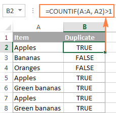
As you can see in the screenshot above, the formula returns TRUE for duplicate values and FALSE for unique values.
Note. If you need to find duplicates in a range of cells rather than in an entire column, remember to lock that range with the $ sign. For example, to search for duplicates in cells A2:A8, use this formula:
=COUNTIF($A$2:$A$8, A2)>1
For a duplicate formula to return something more meaningful than the Boolean values of TRUE and FALSE, enclose it in the IF function and type any labels you want for duplicate and unique values:
=IF(COUNTIF($A$2:$A$8, $A2)>1, "Duplicate", "Unique")
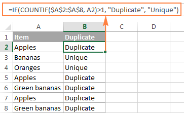
In case, you want an Excel formula to find duplicates only, replace "Unique" with an empty string ("") like this:
=IF(COUNTIF($A$2:$A$8, $A2)>1, "Duplicate", "")
The formula will return "Duplicates" for duplicate records, and a blank cell for unique records:
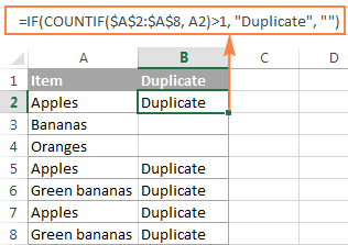
How to search for duplicates in Excel without 1st occurrences
In case you plan to filter or remove duplicates after finding them, using the above formula is not safe because it marks all identical records as duplicates. And if you want to keep the unique values in your list, then you cannot delete all duplicate records, you need to only delete the 2nd and all subsequent instances.
So, let's modify our Excel duplicate formula by using absolute and relative cell references where appropriate:
=IF(COUNTIF($A$2:$A2, $A2)>1, "Duplicate", "")
As you can see in the following screenshot, this formula does not identity the first occurrence of "Apples" as duplicate:
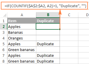
How to find case-sensitive duplicates in Excel
In situations when you need to identify exact duplicates including the text case, use this generic array formula (entered by pressing Ctrl + Shift + Enter):
At the heart of the formula, you use the EXACT function to compare the target cell with each cell in the specified range exactly. The result of this operation is an array of TRUE (match) and FALSE (not match), which is coerced to an array of 1's and 0's by the unary operator (--). After that, the SUM function adds up the numbers, and if the sum is greater than 1, the IF function reports a "Duplicate".
For our sample dataset, the formula goes as follows:
=IF(SUM((--EXACT($A$2:$A$8,A2)))<=1,"","Duplicate")
As shown in the screenshot below, it treats lowercase and uppercase as different characters (APPLES is not identified as a duplicate):

Tip. If you are using Google spreadsheets, the following article might be helpful: How to find and remove duplicates in Google Sheets.
How to find duplicate rows in Excel
If your aim is to dedupe a table consisting of several columns, then you need a formula that can check each column and identify only absolute duplicate rows, i.e. rows that have completely equal values in all columns.
Let's consider the following example. Supposing, you have order numbers in column A, dates in column B, and ordered items in column C, and you want to find duplicate rows with the same order number, date and item. For this, we are going to create a duplicate formula based on the COUNTIFS function that allows checking multiple criteria at a time:
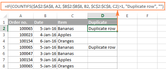
To search for duplicate rows with 1st occurrences, use this formula:
=IF(COUNTIFS($A$2:$A$8,$A2,$B$2:$B$8,$B2,$C$2:$C$8,$C2)>1, "Duplicate row", "")
The following screenshot demonstrates that the formula really locates only the rows that have identical values in all 3 columns. For example, row 8 has the same order number and date as rows 2 and 5, but a different item in column C, and therefore it is not marked as duplicate row:
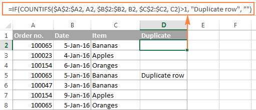
To show duplicate rows without 1st occurrences, make a little adjustment to the above formula:
=IF(COUNTIFS($A$2:$A2,$A2,$B$2:$B2,$B2,$B$2:$B2,$B2,$C$2:$C2,$C2,) >1, "Duplicate row", "")
How to count duplicates in Excel
If you want to know the exact number of identical records in your Excel sheet, use one of the following formulas to count duplicates.
Count instances of each duplicate record individually
When you have a column with duplicated values, you may often need to know how many duplicates are there for each of those values.
To find out how many times this or that entry occurs in your Excel worksheet, use a simple COUNTIF formula, where A2 is the first and A8 is the last item of the list:
=COUNTIF($A$2:$A$8, $A2)
As demonstrated in the following screenshot, the formula counts the occurrences of each item: "Apples" occurs 3 times, "Green bananas" - 2 times, "Bananas" and "Oranges" only once.

If you want to identify 1st, 2nd, 3rd, etc. occurrences of each item, use the following formula:
=COUNTIF($A$2:$A2, $A2)

In a similar manner, you can count the occurrences of duplicated rows. The only difference is that you will need to use the COUNTIFS function instead of COUNTIF. For example:
=COUNTIFS($A$2:$A$8, $A2, $B$2:$B$8, $B2)

Once the duplicate values are counted, you can hide unique values and only view duplicates, or vice versa. To do this, apply Excel's auto-filter as demonstrated in the following example: How to filter out duplicates in Excel.
Count the total number of duplicates in a column(s)
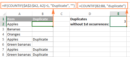
The easiest way to count duplicates in a column is to employ any of the formulas we used to identify duplicates in Excel (with or without first occurrences). And then you can count duplicate values by using the following COUNTIF formula:
=COUNTIF(range, "duplicate")
Where "duplicate" is the label you used in the formula that locates duplicates.
In this example, our duplicate formula takes the following shape:
=COUNTIF(B2:B8, "duplicate")
Another way to count duplicate values in Excel by using a more complex array formula. An advantage of this approach is that it does not require a helper column:
=ROWS($A$2:$A$8)-SUM(IF( COUNTIF($A$2:$A$8,$A$2:$A$8)=1,1,0))
Because it's an array formula, remember to press Ctrl + Shift + Enter to complete it. Also, please keep in mind that this formula counts all duplicate records, including first occurrences:

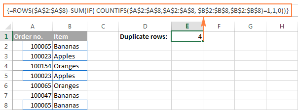
To find the total number of duplicate rows, embed the COUNTIFS function instead of COUNTIF in the above formula, and specify all of the columns you want to check for duplicates. For example, to count duplicate rows based on columns A and B, enter the following formula in your Excel sheet:
=ROWS($A$2:$A$8)-SUM(IF( COUNTIFS($A$2:$A$8,$A$2:$A$8, $B$2:$B$8,$B$2:$B$8)=1,1,0))
How to filter duplicates in Excel
For easier data analysis, you may want to filter your data to only display duplicates. In other situations, you may need the opposite - hide duplicates and view unique records. Below you will find solutions for both scenarios.
How to show and hide duplicates in Excel
If you want to see all duplicates at a glance, use one of the formulas to find duplicates in Excel that better suits your needs. Then select your table, switch to the Data tab, and click the Filter button. Alternatively, you can click Sort & Filter > Filter on the Home tab in the Editing group.
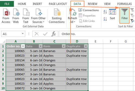
Tip. To have filtering enabled automatically, convert your data to a fully-functional Excel table. Just select all data and press the Ctrl + T shortcut.
After that, click the arrow ![]() in the header of the Duplicate column and check the "Duplicate row" box to show duplicates. If you want to filter out, i.e. hide duplicates, select "Unique" to view only unique records:
in the header of the Duplicate column and check the "Duplicate row" box to show duplicates. If you want to filter out, i.e. hide duplicates, select "Unique" to view only unique records:

And now, you can sort duplicates by the key column to group them for easier analysis. In this example, we can sort duplicate rows by the Order number column:
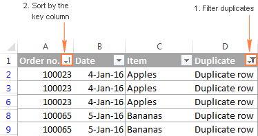
How to filter duplicates by their occurrences
If you want to show 2nd, 3rd, or Nth occurrences of duplicate values, use the formula to count duplicate instances we discussed earlier:
=COUNTIF($A$2:$A2, $A2)
Then apply filtering to your table and select only the occurrence(s) you want to view. For example, you can filter the 2nd occurrences like in the following screenshot:

To display all duplicate records, i.e. occurrences greater than 1, click the filter arrow in the header of the Occurrences column (the column with the formula), and then click Number Filters > Greater Than.
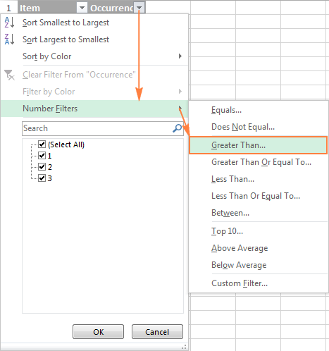
Select "is greater than" in the first box, type 1 in the box next to it, and click the OK button:

In a similar manner, you can show 2nd, 3rd and all subsequent duplicate occurrences. Just type the required number in the box next to "is greater than".
Highlight, select, clear, delete, copy or move duplicates
After you've filtered duplicates like demonstrated above, you have a variety of choices to deal with them.
How to select duplicates in Excel
To select duplicates, including column headers, filter them, click on any filtered cell to select it, and then press Ctrl + A.
To select duplicate records without column headers, select the first (upper-left) cell, and press Ctrl + Shift + End to extend the selection to the last cell.
Tip. In most cases, the above shortcuts work fine and select filtered (visible) rows only. In some rare cases, mostly on very large workbooks, both visible and invisible cells may get selected. To fix this, use one of the above shortcuts first, and then press Alt + ; to select only visible cells, ignoring hidden rows.
How to clear or remove duplicates in Excel
To clear duplicates in Excel, select them, right click, and then click Clear Contents (or click the Clear button > Clear Contents on the Home tab, in the Editing group). This will delete the cell contents only, and you will have empty cells as the result. Selecting the filtered duplicate cells and pressing the Delete key will have the same effect.
To remove entire duplicate rows, filter duplicates, select the rows by dragging the mouse across the row headings, right click the selection, and then choose Delete Row from the context menu.

How to highlight duplicates in Excel
To highlight duplicate values, select the filtered dupes, click the Fill color button ![]() on the Home tab, in the Font group, and then select the color of your choosing.
on the Home tab, in the Font group, and then select the color of your choosing.
Another way to highlight duplicates in Excel is using a built-in conditional formatting rule for duplicates, or creating a custom rule specially tailored for your sheet. Experienced Excel users won't have any problem with creating such a rule based on the formulas we used to check duplicates in Excel. If you are not very comfortable with Excel formulas or rules yet, you will find the detailed steps in this tutorial: How to highlight duplicates in Excel.
How to copy or move duplicates to another sheet
To copy duplicates, select them, press Ctrl + C, then open another sheet (a new or existing one), select the upper-left cell of the range where you want to copy the duplicates, and press Ctrl + V to paste them.
To move duplicates to another sheet, perform the same steps with the only difference that you press Ctrl + X (cut) instead of Ctrl + C (copy).
Duplicate Remover - fast and efficient way to locate duplicates in Excel
Now that you know how to use duplicate formulas in Excel, let me demonstrate you another quick, efficient and formula-free way - Duplicate Remover for Excel.
This all-in-one tool can search for duplicate or unique values in a single column or compare two columns. It can find, select and highlight duplicate records or entire duplicate rows, remove found dupes, copy or move them to another sheet. I think an example of practical use is worth many words, so let's get to it.
How to find duplicate rows in Excel in 2 quick steps
To test the capabilities of our Duplicate Remover add-in, I've created a table with a few hundred rows that looks like follows:

As you see, the table has a few columns. The first 3 columns contain the most relevant information, so we are going to search for duplicate rows based solely on the data in columns A - C. To find duplicate records in these columns, just do the following:
- Select any cell within your table and click the Dedupe Table button on the Excel ribbon. After installing our Ultimate Suite for Excel, you will find it on the Ablebits Data tab, in the Dedupe group.
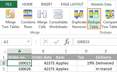
- The smart add-in will pick up the entire table and ask you to specify the following two things:
- Select the columns to check for duplicates (in this example, these are the Order no., Order date and Item columns).
- Choose an action to perform on duplicates. Because our purpose is to identify duplicate rows, I've selected the Add a status column

Apart from adding a status column, an array of other options are available to you:
- Delete duplicates
- Color (highlight) duplicates
- Select duplicates
- Copy duplicates to a new worksheet
- Move duplicates to a new worksheet
Click the OK button and wait for a few seconds. Done!
As you can see in the below screenshot, all of the rows that have identical values in the first 3 columns have been located (first occurrences are not identified as duplicates).

If you want more options to dedupe your worksheets, use the Duplicate Remover wizard that can find duplicates with or without first occurrences as well as unique values. The detailed steps follow below.
Duplicate Remover wizard - more options to search for duplicates in Excel
Depending on a particular sheet you are working with, you may or may not want to treat the first instances of identical records as duplicates. One possible solution is using a different formula for each scenario, as we discussed in How to identify duplicates in Excel. If you are looking for a fast, accurate and formula-free method, try the Duplicate Remover wizard:
- Select any cell within your table and click the Duplicate Remover button on the Ablebits Data tab. The wizard will run and the entire table will get selected.

- On the next step, you are presented with the 4 options to check duplicates in your Excel sheet:
- Duplicates without 1st occurrences
- Duplicates with 1st occurrences
- Unique values
- Unique values and 1st duplicate occurrences
For this example, let's go with the second option, i.e. Duplicates + 1st occurrences:

- Now, select the columns where you want to check duplicates. Like in the previous example, we are selecting the first 3 columns:
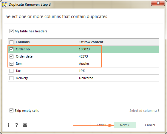
- Finally, choose an action you want to perform on duplicates. As is the case with the Dedupe Table tool, the Duplicate Remover wizard can identify, select, highlight, delete, copy or move duplicates.
Because the purpose of this tutorial is to demonstrate different ways to identify duplicates in Excel, let's check the corresponding option and click Finish:

It only takes a fraction of a second for the Duplicate Remover wizard to check hundreds of rows, and deliver the following result:

No formulas, no stress, no errors - always swift and impeccable results :)
If you are interested to try these tools to find duplicates in your Excel sheets, you are most welcome to download an evaluation version below. Your feedback in comments will be greatly appreciated!
Available downloads
Identify Duplicates - formula examples (.xlsx file)
Ultimate Suite - trial version (.exe file)
 by
by
264 comments
Hi
I'm currently doing keep stock for my store and has many SKUs to fill in. How to automatically add the number of quantity if i double insert the same SKU number in the sheet and it will not appear in the current list that I just keyed-in?
example:
A column B column
SKU QTY
9764454 25
9750936 10
999999 200
9764454 40
much appreciated, thanks~
Hi! To automatically add the number of quantities in column B, a formula must be written in the cell to find the value. For example, this could be the formula VLOOKUP. For example:
=IFERROR(VLOOKUP(A3,$A$1:B2,2,FALSE),"")
To hide the error message if no value is found, the IFERROR function is used.
You can also write and use a VBA macro to do this.
Hi,
Can you help how to identify duplicate data and return with that data with character that would make it unique. For example, I have 123, 123, 123, it will return 123#1, 123#2, 123#3.
Thank you
Hi! You can use COUNTIF function to identify duplicates and determine the ordinal numbers of the duplicates. Try to enter the following formula in cell B1 and then copy it down along the column:
=IF(COUNTIF($A$1:$A$10,A1)>1, A1&"#"&(COUNTIF($A$1:$A$10,A1) - COUNTIF($A2:$A$10,A1)),A1)
Hope this is still an active thread -
I am running into issues when trying to retrieve bottom/top 5 values from a table as the value being used against the table can have duplicates, at the formula always returns the first result.
Example:
John | 97%
Mary | 98%
Matt | 98%
Paul | 100%
Simon | 65%
Jude | 79%
Ashley | 82%
Connor | 79%
Rebecca | 88%
Ryder | 81%
For the above, the bottom 3 would return as follow:
Simon | 65%
Jude | 79%
Jude | 79%
Looking for
Simon | 65%
Jude | 79%
Connor | 79%
Current Formula: =INDEX(A4:A20,MATCH(SMALL(B4:B20,ROWS($A$21:$A23)),B4:B20,0))
I appreciate it!
Hello Kyle!
You can find the answer to your question in this manual: How to find top values with duplicates. Replace the LARGE function in the suggested formulas with SMALL.
In Excel 365, you can use a much simpler FILTER formula that automatically handles ties.
This should solve your task.
Good afternoon.
I am looking through all the comments but couldn't find anything similar to what I am looking for.
I have one tab in Excel that has a list of products (column A) and next to it is the place where the products were sold (column B). I'm looking for a formula that will write for each city individually which product is the best-selling, i.e. which product is repeated the most. Not number of repeats, just a name of a Product. Due to the way of reporting I work, a pivot table is out of the question, it needs to output the result immediately.
The table looks something like this:
Product1 - city1
Product1 - city2
Product1 - city1
Product2 - city1
Product2 - city3
Product4 - city2
Product5 - city4
etc.
Desired result:
city1 - most repeated product is Product1
city2 - most repeated product is Product1
and for all cities like that.
Tried Index, match, mode, all combination, nothing worked.
Thanks in advance.
Hi! To find the most frequent value by the condition, use the FILTER function to get an array of values where the values in column B are equal to cell D1 (for example, "city1"). Then use the INDEX MATCH function to select the most frequently occurring value from the first column of this array. Try to use this formula:
=INDEX(FILTER($A$1:$A$20,$B$1:$B$20=$D$1), MODE(MATCH(FILTER($A$1:$A$20,$B$1:$B$20=$D$1), FILTER($A$1:$A$20,$B$1:$B$20=$D$1),0)))
I have to input data in 15 different sheets in a single workbook of excel. I have to monitor that there should not be input duplicate value. like sheet to sheet check data and should not be a duplicate value in among all sheets. If i input data in next sheet i.e. 16th sheet it should be highlighted that the input value is duplicate.
Hi! Data Validation tool will not be able to automatically validate values on 15 sheets. This can be done using VBA code.
Thanks for the lesson. I'm trying to find exact duplicates in a column of part numbers, and I'm getting duplicates for part numbers that are found in longer versions of themselves. For example, part number 1581H4 is matching as a duplicate to part number 1581H4DP as it is contained in this part number, thought they are not identical. It's like Apple is being matched to Applesauce.
Is there a formula for exact matches up to so many characters, if that would even work?
Thank-you very much. You've been very informative.
Jon
Hello! To get a list of values with a partial match, use the FILTER function. For more information, please read: How to find substring in Excel
=FILTER(B1:B10,ISNUMBER(SEARCH(A1,B1:B10)))
I hope my advice will help you solve your task.
You can ignore this. Seems I've figured out my mistake starting at the wrong cell. Cheers!
I have a list in Excel such as name, surname, street or street address, gender, date of birth.
But the list is very complicated. For example, Gül Sokak is mentioned in lines 1-2-3-4-10-70-99. I want to make a group of all street and avenue names.
Can I group other rows with the same content as any text in a row in a table?
Or I can simply select all the lines belonging to the expression in any line I'm looking for.
Hi! To group rows with the same content, you can sort the data using Excel tools or formulas as described in these articles: Excel: sort by row, by column names and in custom order and Excel SORT function - auto sort data using formula.
To get all rows with specific content, you can use the FILTER function.
I hope my advice will help you solve your tas
I have a data set that has the reference # in column A with specific information listed in subsequent columns. Unfortunately, the column that lists the primary and co investigators on each project lists them over two or more rows, leaving me with multiple reference ID#'s in column A for the same project. These repeats are making it impossible for me to merge other bits of information. Is there a way I can remove the multiple appearance of the reference # and replace it with blank cells so that it does not remove the entire row?
Hi! I'd recommend you to take a look at our Remove Duplicates tool that can help you find and remove duplicates from the table. It helps you solve this task in a few clicks. This tool is available as a part of our Ultimate Suite for Excel that you can install in a trial mode and check how it works for free.
hi. i want to identify 1st, 2nd, 3rd, etc. occurrences of each item in table , i follow the way you say but when i add a new row to table my range changes..what can i do for this problem?
Hi! Please clarify your specific problem or provide additional information to understand what you need. It might help if you use absolute references. Read more: Relative and absolute cell reference: why use $ in Excel formula
Hi,
I have a big datasheet. We run samples matched by MRN #. For example ID#1 has MRN 345 with label T and ID#2 has MRN 345 with Label N. If MRN 345 was run before and we have to run it again. the labels have to be T2 and Nrpt. Is there a way to do that in excel?
Hi! Please clarify your specific problem or provide additional details to highlight exactly what you need. As it's currently written, it's hard to tell exactly what do you want to do.
Hello Team:
In this forum you solve my many problems thanks,
Now I have also another problem, as i share the data which is duplicate values in a single column, these are duplicates and only find it
manually, not any formula or conditional formatting,
I need a formula to find the duplicate in the following text strings which is in a single column,the number shows how much time it is repeated, I find it manually
it is very large data file, so i need your help,
Thanks a lot advance:
1 8041-GTN to DC-44 Firdous Market
1 FZRD: OLT-1 to C-5 Pak Arab Society
1 8061-ARZ (2/0/7) to C-3/4 Bhobhtian Chowk
2 FRZD: OLT-1 to C-5 Pak Arab Society
1 SMD: MSAG-37 GOR-III to C-32 Cricket House GOR-II & C-3 Rehmania Park
1 SMD: OLT-1 to C-13 Truck Stand Adda
2 8061-ARZ (2/0/7) to C-3/4 Bhobhtian Chowk
4 8061-ARZ (11/0/7) to C-3/4 Bhobtian Chowk Defence Road
2 SMD: OLT-1 to C-13 Truck Stand Adda
1 FZRD: FZRD OLT-1 to MSAG-58 Near Advance Fashion
2 8041-GTN to DC-44 Firdous Market
3 8061-ARZ (2/0/7) to C-3/4 Bhobhtian Chowk Defence Road
2 FZRD: OLT-1 to MSAG-58 near Advance Fashion
1 BTN: OLT-1 to Leads Club Defence Road
8041-GTN to 8052-GLB
1 MLRD: OLT-1 to C-22 H#106 Awan Town
2 BTN: OLT-1 to Leads Club Defence Road
2 MLRD: OLT-1 to C-22 H#106 Awan Town
2 SMD: MSAG-37 GOR-III to C-3 Rehmania Park & C-32 Cricket House GOR-II
Please use this
=SUMPRODUCT(--($A:$A=A2))
Hi! From your question, the desired result is not very clear. If I understand the question correctly, to calculate the number of duplicates in a column, use the recommendations from the paragraph above in the article: How to count duplicates in Excel. If that's not what you want, describe exactly what result you wanted.
Sir,
Thanks a lot for your response, actually I share my data that these text strings are duplicate but the problems that they are occurred in the
data that their sequence is not same but they are the same stations name and the same fault which are in a weekly fault report, I am searching manually and then pulled out from the report, I need a formula to find it and then i pulled out,
For example if you see the Sr.no. 1&11 are same fault but only the sequence is changed, sr.no.2&4,sr#3&7 and all other also, this a huge data and i
pulled the same fault occurance manuallu, I shall be very thankful to you for your help thanks a lot:
8041-GTN to DC-44 Firdous Market 1
FZRD: OLT-1 to C-5 Pak Arab Society 2
8061-ARZ (2/0/7) to C-3/4 Bhobhtian Chowk 3
FRZD: OLT-1 to C-5 Pak Arab Society 4
SMD: MSAG-37 GOR-III to C-32 Cricket House GOR-II & C-3 Rehmania Park 5
C-13 Truck Stand Adda to SMD: OLT-1 6
Bhobhtian Chowk to 8061-ARZ (2/0/7) and C-3/4 7
8061-ARZ (11/0/7) to C-3/4 Bhobtian Chowk Defence Road 8
SMD: OLT-1 to C-13 Truck Stand Adda 9
FZRD: FZRD OLT-1 to MSAG-58 Near Advance Fashion 10
Firdous Market to 8041-GTN DC-44 11
8061-ARZ (2/0/7) to C-3/4 Bhobhtian Chowk Defence Road 12
FZRD: OLT-1 to MSAG-58 near Advance Fashion 13
Hi! Sorry, I do not fully understand the task. As it's currently written, it's hard to tell exactly what you're asking. I don't see "sr.no." in your data. As I wrote before, specify exactly what result you want from the data you wrote.
Sir,
I am sorry, you do not understand what I want, as a already explain I share my data that these text strings are duplicate but the problems that they are occurred in the data that their sequence is not same but the same fault which are in a weekly fault report, I am searching manually and then pulled out from the report, I need a formula to find it and then i pulled out, If that are same I can use conditional formatting.
For example if you see the Sr.no. 1&11 are same fault but only the sequence is changed, sr.no.2&4,sr#3&7 and all other also, this a huge data and i pulled the same fault occurance manuallu, I shall be very thankful to you for your help thanks a lot:
SR.NO TEXT STRINGS
1 8041-GTN to DC-44 Firdous Market
2 FZRD: OLT-1 to C-5 Pak Arab Society
3 8061-ARZ (2/0/7) to C-3/4 Bhobhtian Chowk
4 FRZD: OLT-1 to C-5 Pak Arab Society
5 SMD: MSAG-37 GOR-III to C-32 Cricket House GOR-II & C-3 Rehmania Park
6 C-13 Truck Stand Adda to SMD: OLT-1
7 Bhobhtian Chowk to 8061-ARZ (2/0/7) and C-3/4
8 8061-ARZ (11/0/7) to C-3/4 Bhobtian Chowk Defence Road
9 SMD: OLT-1 to C-13 Truck Stand Adda
10 FZRD: FZRD OLT-1 to MSAG-58 Near Advance Fashion
11 Firdous Market to 8041-GTN DC-44
12 8061-ARZ (2/0/7) to C-3/4 Bhobhtian Chowk Defence Road
13 FZRD: OLT-1 to MSAG-58 near Advance Fashion
This is the third time you repeat the same thing and don't give an example of the result you want to get from the data you wrote. You have written 13 values. What result do you want to get from them? If you need to count duplicates, read the paragraph above: How to count duplicates in Excel
Thanks a lot sir,
I show this again and again that I want to get duplicate value like these text strings
I have a spreadsheet with lots of rows of data and 5 columns, named "Guests", "Guest type", "Status", "No of Pax" and "Type of Meal".
What I'm looking for is how to find the duplicated guests and transpose those names with the sum of total pax, based on the criteria of the "Guest type", "Status" and "Type of Meal".
I hope I can make myself clear enough so you can help me out.
The final result would have the name of the client in one column and the total of meals based on those criteria on another column.
Thanks in advance.
Silvio
Hello! To calculate the total of meals based on the three criteria, use the COUNTIFS function. See the instructions and examples in this article: Excel COUNTIFS and COUNTIF with multiple AND / OR criteria. I hope it’ll be helpful.
Thank you for your reply. I basically know I to use the countif and countifs, but what I wanted is how to find the duplicate names, and when they are found how to automatically transpose those names plus the results of the criteria to different columns.
Say for example I have on column A 100 names with several that are duplicates (repeated guests). They all have a type of guest assigned, a status (confirmed, cancelled), number of persons assigned to that guest and type of meals (breakfast, lunch or dinner).
I only want to extract the information of duplicated names plus the total sum of persons assigned to those names, based on the criteria chosen, say type of, confirmed or cancelled and type of meals.
I hope you understand what I'm looking for.
Thank you
Hi! You can get the list of duplicates to a separate column using any of the methods recommended in the article above. You can also extract a list of unique values from column A as described in this guide: Excel UNIQUE function - fastest way to find unique values.
Then in the next column, for each of the clients, do a calculation using the COUNTIFS function.
This is the formula I use to count number of meals based on those criteria
=SUMIFS($H$2:$H$5000;$C$2:$C$5000;"Passant";$G$2:$G$5000;"Confirmed";$J$2:$J$5000;"Dinner")
It works pretty well. Now I just want to identify from the list of names which are the clients that had been several times and based on the same criteria how many times they had dinner or a different meal.
Hi! You can count the number of customers by certain criteria using the COUNTIFS function.
This is great information, but not sure if it addresses what I need to achieve:
I have a multi-level/hierarchial Bill of Materials of a product with multiple components, some sharing the same sub-components:
One column is the item number, that specifies the hierarchy, i.e. 1, 1.1, 1.1.1, 1.1.2... 1.1.10 etc
Other columns specify Description, Part Number, Material, and so on
The last column is the Quantity column
I want to be able to find parts with duplicate part numbers in the table, and return the Total Quantity of these shared parts somehow; possibly in another table/row, or *maybe* better a Total Quantity column
Hello!
If I understand the problem correctly, you can calculate the number of identical item numbers using the formulas from this guide: How to count duplicates in Excel.
I hope it’ll be helpful. If this is not what you wanted, please describe the problem in more detail.
Hi
I have list with thousands Products list
A- have Product Code
B Have names
C Have QTY
Now i need to Put price for each item in no 4 same items is repeated many times is their a way to put Price in all same items at Once?
Hi!
To quickly find the price for each of the 4 products and insert it into the table, use the VLOOKUP function. Please have a look at this article Excel VLOOKUP function tutorial with formula examples.
Dears,
I have a lot of paragraphs "in 2000 Rows" in the excel sheet and I want to extract value from them in specific line or to get the duplication from specific line.
Am doing analysis for debtors then i have two listings ,which formula can i use to find duplicates from last year listing to this year listing
Hi!
I think you will find the answer in this article: How to compare two columns in Excel for matches and differences.
Hi Guys, thanks for this very useful website and forum!
I have a weekly report showing a list of incoming calls to a ring group in a queue, with date (DD/MM/YYYY HH:MM:SS), caller ID (phone number), the agent id (extension number of receiving agent), and the status (answered, no answer, busy).
I am trying to work out the Call Abandon Rate so I need to identify a formula that looks for blocks of entries with same date and same phone number, and then refers to the 'status' column to determine whether at least one of the rows in the array is flagged as 'answered'.
Struggling to find a formula that does the job. Would anyone be able to assist?
Thanks, Tiziana
Hello!
If I understand your task correctly, use the FILTER function to get all the records by the criteria you specified
=(FILTER($D$2:$D$10,(--(INT($A$2:$A$10)=INT(A2)))* (--($B$2:$B$10=B2))* (--($D$2:$D$10="answered")),"")<>"")
Thanks Alexander, that works brilliantly!
Unfortunately I am getting a series of '#SPILL!' errors however, and since I am working on a rather large data set (7000+ rows), I am wondering whether there is a way for me to prevent this error from occurring? Otherwise I'd be left with manually deleting the obstructing cells, which could be very time consuming.
Thanks again, Tiziana
Hi!
Write the formula so it will not interfere with other data cells. For more information, read #SPILL! error in Excel - what it means and how to fix.
Thanks Alexander, I will check and let you know in case of difficulties!
Hi Alexander, I read through and applied the solution that's outlined on the indicated page: #SPILL! error in Excel - what it means and how to fix. The issue I'm facing however, is that clearing the obstructed cells for this data set of just over 6000 rows is proving to be fairly laborious. The SPILL# error appears at around the 75th row, and continues to reappear frequently thereafter. Would you know how else this may be tackled please? Thanks !
Hi!
Unfortunately, there are no other solutions besides clearing the cells. Either move the cell with the formula to an empty space or to another worksheet.
I have a column that consists of 100+ rows than contain several repeated values within a single cell, separated by commas:
example:
Cell A1: apple, apple, orange, banana, banana
Cell A2: orange, apple, banana
Cell A3: orange, orange, banana
. Is there a way I can have another column that indicates whether a single cell consist of "duplicates" (Cell A1 and A3) and "no duplicates." (Cell A2)?
Hello!
Your problem cannot be solved with a single formula. You can create a copy of this column. Then use the Remove Duplicate Substrings Tool to remove duplicates from the text cells in that column. Then compare the two columns and you will see differences where there were duplicates.
For more information, please read: Compare two columns for matches and differences.
Remove Duplicate Substrings Tool is available as a part of our Ultimate Suite for Excel that you can install in a trial mode and check how it works for free.
When I copy and paste the duplicate expression =COUNTIF(A:A, A2)>1 it works perfectly in my spreadsheet. When I type it in manually it never works correctly?
I have 4 line items for duplicate and I did below formula to find them.
but now for $$ value, I only need one line item (mostly recent line), how can i formula this?
Formula for duplicate: =COUNTIFS($A$2:$100,@A:A)
For amount, I need last row from four duplicates.
AMT:
7000
7000
-7000
7000
Hi!
To find the position of the last match in the list, use the XMATCH function
=XMATCH(C1,A1:A10,0,-1)
Hope this is what you need.