The tutorial explains how to lock a cell or certain cells in Excel to protect them from deleting, overwriting or editing. It also shows how to unlock individual cells on a protected sheet by a password, or allow specific users to edit those cells without password. And finally, you will learn how to detect and highlight locked and unlocked cells in Excel.
In last week's tutorial, you learned how to protect Excel sheets to prevent accidental or deliberate changes in the sheet contents. However, in some cases you may not want to go that far and lock the entire sheet. Instead, you can lock only specific cells, columns or rows, and leave all other cells unlocked.
For example, you can allow your users to input and edit the source data, but protect cells with formulas that calculate that data. In other words, you may want to only lock a cell or range that shouldn't be changed.
How to lock cells in Excel
Locking all cells on an Excel sheet is easy - you just need to protect the sheet. Because the Locked attributed is selected for all cells by default, protecting the sheet automatically locks cells.
If you don't want to lock all cells on the sheet, but rather want to protect certain cells from overwriting, deleting or editing, you will need to unlock all cells first, then lock those specific cells, and then protect the sheet.
The detailed steps to lock cells in Excel 365 - 2010 follow below.
1. Unlock all cells on the sheet
By default, the Locked option is enabled for all cells on the sheet. That is why, in order to lock certain cells in Excel, you need to unlock all cells first.
- Press Ctrl + A or click the Select All button
 to select the entire sheet.
 - Press Ctrl + 1 to open the Format Cells dialog (or right-click any of the selected cells and choose Format Cells from the context menu).
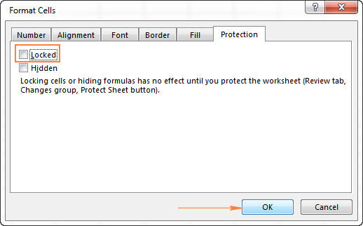
- In the Format Cells dialog, switch to the Protection tab, uncheck the Locked option, and click OK.
2. Select cells, ranges, columns or rows you want to protect
To lock cells or ranges, select them in a usual way by using the mouse or arrow keys in combination with Shift. To select non-adjacent cells, select the first cell or a range of cells, press and hold the Ctrl key, and select other cells or ranges.
To protect columns in Excel, do one of the following:
- To protect one column, click on the column's letter to select it. Or, select any cell within the column you want to lock, and press Ctrl + Space.
- To select adjacent columns, right click on the first column heading and drag the selection across the column letters rightwards or leftwards. Or, select the first column, hold down the Shift key, and select the last column.
- To select non-adjacent columns, click on the first column's letter, hold down the Ctrl key, and click the headings of other columns you want to protect.
To protect rows in Excel, select them in a similar manner.
To lock all cells with formulas, go to the Home tab > Editing group > Find & Select > Go To Special. In the Go To Special dialog box, check the Formulas radio button, and click OK. For the detailed guidance with screenshots, please see How to lock and hide formulas in Excel.
3. Lock selected cells
With the required cells selected, press Ctrl + 1 to open the Format Cells dialog (or right-click the selected cells and click Format Cells), switch to the Protection tab, and check the Locked checkbox.

4. Protect the sheet
Locking cells in Excel has no effect until you protect the worksheet. This can be confusing, but Microsoft designed it this way, and we have to play by their rules :)
On the Review tab, in the Changes group, click the Protect Sheet button. Or, right click the sheet tab and select Protect Sheet… in the context menu.

You will be prompted to enter the password (optional) and select the actions you want to allow users to perform. Do this, and click OK. You can find the detailed instructions with screenshots in this tutorial: How to protect a sheet in Excel.
Done! The selected cells are locked and protected from any changes, while all other cells in the worksheet are editable.
If you are working in Excel web app, then see how to lock cells for editing in Excel Online.
How to unlock cells in Excel (unprotect a sheet)
To unlock all cells on a sheet, it is sufficient to remove the worksheet protection. To do this, right-click the sheet tab, and select Unprotect Sheet… from the context menu. Alternatively, click the Unprotect Sheet button on the Review tab, in the Changes group:

For more information, please see How to unprotect an Excel sheet.
As soon as the worksheet is unprotected, you can edit any cells, and then protect the sheet again.
If you want to allow users to edit specific cells or ranges on a password-protected sheet, check out the following section.
How to unlock certain cells on a protected Excel sheet
In the first section of this tutorial, we discussed how to lock cells in Excel so that no one even yourself can edit those cells without unprotecting the sheet.
However, sometimes you may want to be able to edit specific cells on your own sheet, or let other trusted users to edit those cells. In other words, you can allow certain cells on a protected sheet to be unlocked with password. Here's how:
- Select the cells or ranges you want to unlock by a password when the sheet is protected.
- Go to the Review tab > Changes group, and click Allow Users to Edit Ranges.

Note. This feature is available only in an unprotected sheet. If the Allow Users to Edit Ranges button is greyed out, click the Unprotect Sheet button on the Review tab.
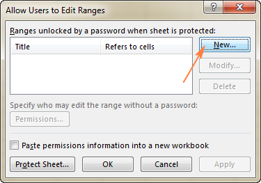
- In the Allow Users to Edit Ranges dialog window, click the New… button to add a new range:
- In the New Range dialog window, do the following:
- In the Title box, enter a meaningful range name instead of the default Range1 (optional).
- In the Refers to cells box, enter a cell or range reference. By default, the currently selected cell(s) or range(s) are included.
- In the Range password box, type a password. Or, you can leave this box empty to allow everyone to edit the range without password.
- Click the OK button.

Tip. In addition to, or instead of, unlocking the specified range by a password, you can give certain users the permissions to edit the range without password. To do this, click the Permissions… button in the lower left corner of the New Range dialog and follow these guidelines (steps 3 - 5).
- The Confirm password window will appear and prompt you to re-type the password. Do this, and click OK.
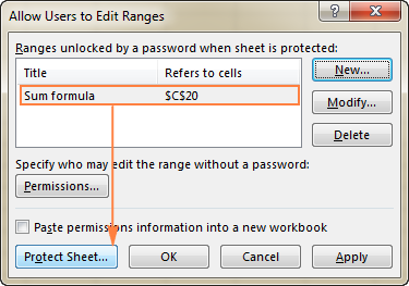
- The new range will get listed in the Allow Users to Edit Ranges dialog. If you want to add a few more ranges, repeat steps 2 - 5.
- Click the Protect Sheet button at the button of the window to enforce the sheet protection.
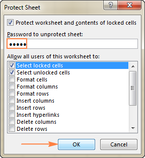
- In the Protect Sheet window, type the password to unprotect the sheet, select the check boxes next to the actions you want to allow, and click OK.
Tip. It is recommended to protect a sheet with a different password than you used to unlock the range(s).
- In the password confirmation window, re-type the password and click OK. That's it!
Now, your worksheet is password protected, but specific cells can be unlocked by the password you supplied for that range. And any user who knows that range password can edit or delete the cells contents.
Allow certain users to edit selected cells without password
Unlocking cells with password is great, but if you need to frequently edit those cells, typing a password every time can be a waste of your time and patience. In this case, you can set up permissions for specific users to edit some ranges or individual cells without password.
Note. This features works on Windows XP or higher, and your computer must be on a domain.
Assuming that you have already added one or more ranges unlockable by a password, proceed with the following steps.
- Go to the Review tab > Changes group, and click Allow Users to Edit Ranges.
Note. If the Allow Users to Edit Ranges is grayed out, click the Unprotect Sheet button to remove the worksheet protection.
- In the Allow Users to Edit Ranges window, select the range for which you want to change the permissions, and click the Permissions… button.
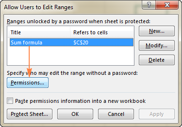
Tip. The Permissions… button is also available when you are creating a new range unlocked by a password.
- The Permissions window will open, and you click the Add… button.
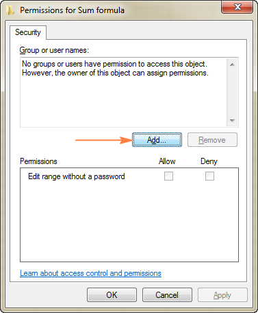
- In the Enter the object names to select box, enter the names of the user(s) whom you want to allow to edit the range.
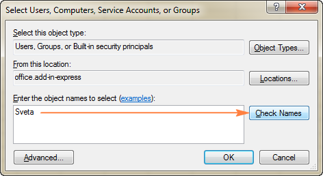
To see the required name format, click the examples link. Or, simply type the user name as it is stored on your domain, and click the Check Names button to verify the name.
For example, to allow myself to edit the range, I've typed my short name:
Excel has verified my name and applied the required format:
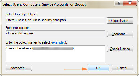
- When you've entered and validated the names of all users to whom you want to give the permissions to edit the selected range, click the OK button.
- Under Group or user names, specify the permission type for each user (either Allow or Deny), and click the OK button to save the changes and close the dialog.
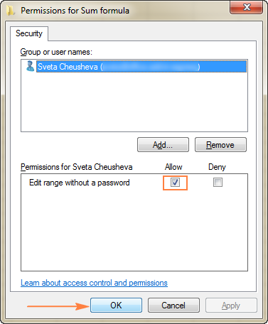
Note. If a given cell belongs to more than one range unlocked by a password, all users who are authorized to edit any of those ranges can edit the cell.
How to lock cells in Excel other than input cells
When you've put a lot of effort in creating a sophisticated form or calculation sheet in Excel, you will definitely want to protect your work and prevent users from tampering with your formulas or changing data that shouldn't be changed. In this case, you can lock all cells on your Excel sheet except for input cells where your users are supposed to enter their data.
One of possible solutions is to use the Allow Users to Edit Ranges feature to unlock selected cells, as demonstrated above. Another solution could be modifying the built-in Input style so that it not only formats the input cells but also unlocks them.
For this example, we are going to use an advanced compound interest calculator that we created for one of the previous tutorials. This is how it looks like:
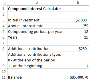
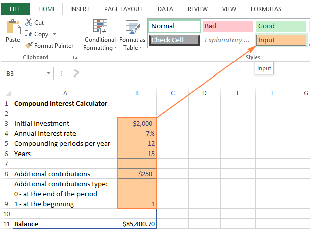
Users are expected to enter their data in cells B2:B9, and the formula in B11 calculates the balance based on the user's input. So, our aim is to lock all cells on this Excel sheet, including the formula cell and fields' descriptions, and leave only the input cells (B3:B9) unlocked. To do this, perform the following steps.
- On the Home tab, in the Styles group, find the Input style, right click it, and then click Modify….
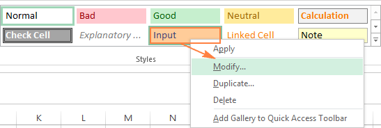
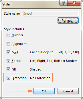
- By default, Excel's Input style includes information about the font, border and fill colors, but not the cell protection status. To add it, just select the Protection checkbox:
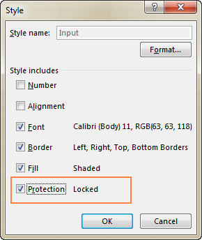
Tip. If you want only to unlock input cells without changing cell formatting, uncheck all boxes on the Style dialog window other than the Protection box.
- As you can see in the screenshot above, Protection is now included in the Input style, but it's set to Locked, while we need to unlock input cells. To change this, click the Format… button in the upper right corner of the Style window.
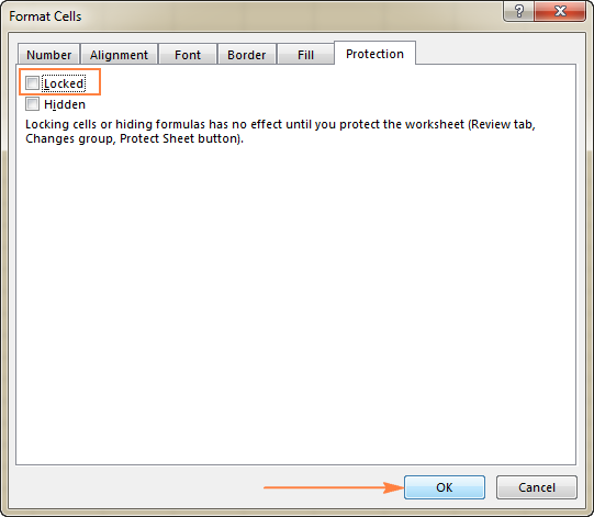
- The Format Cells dialog will open, you switch to the Protection tab, uncheck the Locked box, and click OK:
- The Style dialog window will update to indicate the No Protection status like shown below, and you click OK:
- And now, select the input cells on your sheet and click the Input style button on the ribbon. The selected cells will get both formatted and unlocked at the same time:
- As you may remember, locking cells in Excel has no effect until the sheet protection is turned on. So, the last thing left for you to do is to go to the Review tab > Changes group, and click the Protect Sheet button.
If Excel's Input style does not suit you for some reason, you can create your own style that unlocks selected cells, the key point is to select the Protection box and set it to No Protection, as demonstrated above.
How to find and highlight locked / unlocked cells on a sheet
If you have been locking and unlocking cells on a given spreadsheet multiple times, you may have forgotten which cells are locked and which are unlocked. To quickly find locked and unlocked cells, you can use the CELL function, which returns information about the formatting, location and other properties if a specified cell.
To determine the protection status of a cell, enter the word "protect" in the first argument of your CELL formula, and a cell address in the second argument. For example:
=CELL("protect", A1)
If A1 is locked, the above formula returns 1 (TRUE), and if it's unlocked the formula returns 0 (FALSE) as demonstrated in the screenshot below (the formulas are in cells B1 and B2):

It cannot be easier, right? However, if you have more than one column of data, the above approach is not the best way to go. It would be far more convenient to see all locked or unlocked cells at a glance rather than sorting out numerous 1's and 0's.
The solution is to highlight locked and/or unlocked cells by creating a conditional formatting rule based on the following formulas:
- To highlight locked cells:
=CELL("protect", A1)=1 - To highlight unlocked cells:
=CELL("protect", A1)=0
Where A1 is the leftmost cell of the range covered by your conditional formatting rule.
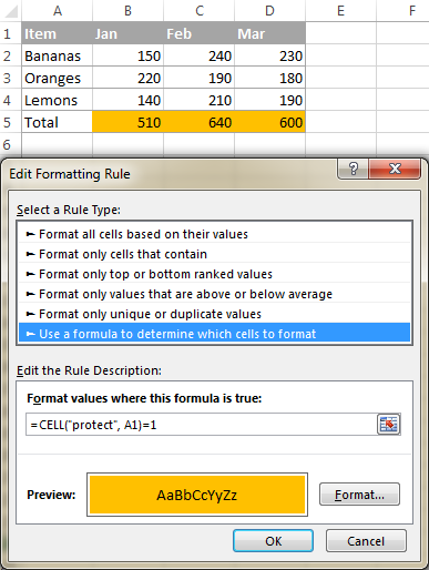
As an example, I've created a small table and locked cells B2:D2 that contain SUM formulas. The following screenshot demonstrates a rule that highlights those locked cells:
Note. The conditional formatting feature is disabled on a protected sheet. So, be sure to turn off the worksheet protection before creating a rule (Review tab > Changes group > Unprotect Sheet).
If you don't have much experience with Excel conditional formatting, you may find the following step-by-step instructions helpful: Excel conditional formatting based on another cell value.
This is how you can lock one or more cells in your Excel sheets. If someone knows any other way to protect cells in Excel, your comments will be truly appreciated. I thank you for reading and hope to see you on our blog next week.
 by
by
64 comments
If you have been locking and unlocking cells on a given spreadsheet multiple times, you may have forgotten which cells are locked and which are unlocked. To quickly find locked and unlocked cells, you can use the CELL function, which returns information about the formatting, location and other properties if a specified cell.
To determine the protection status of a cell, enter the word "protect" in the first argument of your CELL formula, and a cell address in the second argument. For example:
=CELL("protect", A1)
If A1 is locked, the above formula returns 1 (TRUE), and if it's unlocked the formula returns 0 (FALSE) as demonstrated in the screenshot below (the formulas are in cells B1 and B2):
Use the CELL function to determine the protection status of a cell.
It cannot be easier, right? However, if you have more than one column of data, the above approach is not the best way to go. It would be far more convenient to see all locked or unlocked cells at a glance rather than sorting out numerous 1's and 0's.
The solution is to highlight locked and/or unlocked cells by creating a conditional formatting rule based on the following formulas:
To highlight locked cells: =CELL("protect", A1)=1
To highlight unlocked cells: =CELL("protect", A1)=0
Where A1 is the leftmost cell of the range covered by your conditional formatting rule.
Nice
nice
Amazing. Thanks for your help!
How do I lock merged cells? I get an error when trying to do so. Please and thank you.
You are explaining the best way !!!
thank you so much!!!
My way -
To lock / unlock cells - sheet must ne unprotected - home tab - click format icon (in cells section) - Lock cells (or unlock if locked) - and can R-click on Lock Cell and add to quick access
To know which cells are locked / unlocked I use conditional formatting - formula: =cell("protect",cell-range-etc.)=0 - then setting the format (can be a colour to the text or the cell fill - could be a box round the protected cell(s) - could be say italics on all protected cells (f =1 prob.)
I have a spreadsheet where I locked the cells that had formulas or historical data, but left the input cells unlocked. However Excel won't allow the user to change the fill color of the unlocked input cells. Is there a way to fix this?
I have a worksheet which is used to randomly select one officer out of all officer in shift to go for medical check within half n hour of shift start.
Regulatory bodies want the sheet to be locked for further change, after all the names are entered for the shift officers.
Once all names are entered, the sheet is required to be locked for further manipulations.
How to do this?
Hi Svetlana
Can you help me to lock an exel sheet with ckeckbox content. But when they uncheck the content on the line, the next line opens?
I am trying to accomplish the following:
I have a document where depending one what is selected in A2 - cells are highlighted, based on conditional formatting, to either stay the same or be grayed out. If they are grayed out they do not need to be filled out based on what was selected in A2. Is there a way to protect only the cells that are grayed out. The problem I am having with this is that what needs to be protected changes every time something different is selected in A2. Is there a way to easily protect only grayed out cells - even if what cells are gray changes every time? Please let me know.
Hi!
You can conditionally protect cells using a VBA macro. Excel's conditional formatting can't do this.
?
Lifesaver! Well-written article!
Thanks. So many great, useful options! For my project, I need to accomplish these specifics:
- Send my designed worksheet individually to users whom I progressively select over a one-week period. I wish to invite their input one at a time as each "qualifies." Email is fine - they are all in my network.
- Each user will "qualify" for a certain number of available (unused) cells in a fairly large range. So if you "earned" 5 cells of input, I would invite you and give you the freedom to pick whichever five available cells you prefer in said range.
- I don't want any newly invited user to have access to any already-filled cells. In other words, the person invited AFTER you have filled your five should not have the ability to modify/erase any of your five. They will only have access to the remaining unused cells in that field. And then theirs are also locked from the next person.
- Process continues until all cells are filled.
Which of the options/methods would be the best/most efficient way to set that up? Thank you so much!
Dave
Hi
I'd like to unlock ranges for separate users so they can change their work calendar:
like => range 1 for Erik only
range 2 for Andy only
....
so Andy shouldn't be able to change the range of Erik. I've tried to give permissions & deny permissions for the specific users. but NOT WORKED .
MAYBE DUE TO A DOMAIN ISSUE OR SOMETHING?
PLEASE HELP???
The above method should work as defined. It sounds like a domain issue. you should be able to "search" for the person's username and click on it to set that person's specific permissions.
Oh! you have to enter some sort of password for each permission exception you add. It's a pain to set up initially, but once it's set up it should work just fine
Hi,
i have a shared excel sheet among my employees as below,
No Opportunity Employee Value
1 Customer A dinushab@abc.lk $345,192.00
2 Customer B Chinthakak@abc.lk $456,789.00
3 Customer C kavindus@abc.lk $65,347.00
4 Customer A sandalikav@abc.lk $23,451,246.00
5 Customer B kavindus@abc.lk $98,709,800.00
I want to allow a particular employee to edit the value and customer and allow others to view ony. please note that all employees are using office 365 user accounts. kindly support me
Whatevery help I need in Office i always come to this site first - it never disappoints!
Thank you, Rachel! We will try to keep it that way :)
Thanks a lot! Much appreciated.
Hi!
I hope you can help me.
I know how to lock and unlock cells.
I want to lock a Data Validation cell )that pulls data from a list on a separate, locked spreadsheet) so that only the pull down options are possible.
When I leave this cell unlocked on a protected sheet it is still possible to eliminate the data validation completely and leave blank or enter a different value. If I lock the cell then the pull down menu does not work.
Help!
On a separate note, I see that if I lock all cells (ie by choosing the top left corner) on a worksheet the "math" within cells is not visible. The only way I can find to get around this is to leave at least one cell unlocked. Comments?
In excel data table, if the Sheet Protection is turned on, the option of new in data entry form gets turned off. How to solve this issue. Thanks
Hi Svetlana,
Can I give "edit access of specific areas" to specific users on Excel (without the password option; inserting various passwords)?
For instance:
A1 to A14 (edit access) to user "X"
B1 to B14 (edit access) to user "Y"
User "X" can see "B1 to B14" but can't edit it.
Similarly, the user "Y" can see "A1 to A14" but can't edit it.
It means users can view the entire sheet but can edit the limited section (given permission).