The tutorial shows how to safely merge rows in Excel in 4 different ways: merge multiple rows without losing data, combine duplicate rows, repeatedly merge blocks of rows, and copy matching rows from another table based on one or more common columns.
Merging rows in Excel is one of the most common tasks that all of us need to perform every now and then. The problem is that Microsoft Excel does not provide a reliable tool to do this. For example, if you try to combine two or more rows using the built-in Merge & Center button, you will end up with the following error message:
"The selection contains multiple data values. Merging into one cell will keep the upper-left most data only."

Clicking OK will merge the cells but only keep the value of the first cell, all other data will be gone. So, obviously we need a better solution. This article describes several methods that will let you merge multiple rows in Excel without losing any data.
How to merge rows in Excel without losing data
The task: you have a database where each row contains certain details such as product name, product key, customer name and so on. What we want is to combine all the rows related to a particular order like shown below:
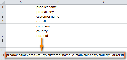
There are two ways to achieve the desired result:
Merge multiple rows using formulas
To joint the values from several cells into one, you can use either the CONCATENATE function or concatenation operator (&). In Excel 2016 and higher, you can also use the CONCAT function. Any way, you supply cells as references and type the desired delimiters in-between.
Merge rows and separate the values with comma and space:
=CONCATENATE(A1,", ",A2,", ",A3)
=A1&", "&A2&", "&A3
Merge rows with spaces between the data:
=CONCATENATE(A1," ",A2," ",A3)
=A1&" "&A2&" "&A3
Combine rows and separate the values with commas without spaces:
=CONCATENATE(A1,A2,A3)
=A1&","&A2&","&A3
In practice, you may often need to concatenate more cells, so your real-life formula is likely to be a bit longer:
=CONCATENATE(A1,", ",A2,", ",A3,", ",A4,", ",A5,", ",A6,", ",A7,", ",A8)
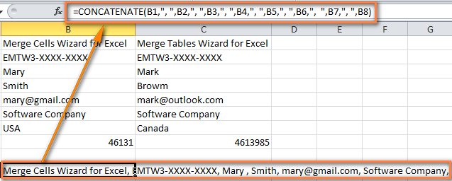
Now you have several rows of data merged into one row. But your combined rows are formulas. To convert them to values, use the Paste Special feature as described in How to replace formulas with their values in Excel.
Combine rows in Excel with Merge Cells add-in
The Merge Cells add-in is a multi-purpose tool for joining cells in Excel that can merge individual cells as well as entire rows or columns. And most importantly, this tool keeps all the data even if the selection contains multiple values.
To merge two or more rows into one, here's what you need to do:
- Select the range of cells where you want to merge rows.
- Go to the Ablebits Data tab > Merge group, click the Merge Cells arrow, and then click Merge Rows into One.

- This will open the Merge Cells dialog box with the preselected settings that work fine in most cases. In this example, we only change the separator from the default space to line break, as shown in the screenshot below:

- Click the Merge button and observe the perfectly merged rows of data separated with line breaks:

How to combine duplicate rows into one (keeping unique values only)
The task: you have some Excel database with a few thousand entries. The values in one column are essentially the same while data in other columns are different. Your goal is to combine data from duplicate rows based on a certain column, making a comma separated list. Additionally, you may want to merge unique values only, omitting duplicates and skipping empty cells.
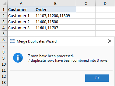
The screenshot below shows what we are trying to achieve.
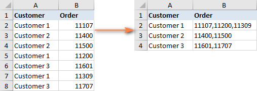
The prospect of finding and merging duplicate rows manually is definitely something you'd want to avoid. Meet the Merge Duplicates add-in that turns this time-consuming and cumbersome chore into a quick 4-steps process.
- Select the duplicate rows you want to merge and run the Merge Duplicates wizard by clicking its button on the ribbon.

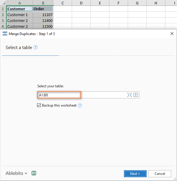
- Make sure your table is selected correctly and click Next. It is wise to keep the Create a backup copy option checked, especially if you are using the add-in for the first time.
- Select the key column to check for duplicates. In this example, we select the Customer column because we want to combine rows based on customer name.
If you want to skip empty cells, be sure to select this option and click Next.

- Choose the columns to merge. In this step, you select the columns whose data you want to combine data and specify the delimiter: semicolon, comma, space, line break, etc.
Two additional options in the upper part of the window let you:
- Delete duplicate values while combining the rows
- Skip empty cells
When done, click the Finish button.

In a moment, all the data from duplicate rows are merged into one row:
How to repeatedly merge blocks of rows into one row
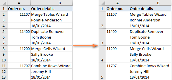
The task: you have an Excel file with information about the recent orders and each order takes 3 lines: product name, customer name and date of purchase. You would like to merge every three rows into one, i.e. repeatedly merge the blocks of three rows.
The following image show what we are looking for:
If there are only few entries to be combined, you can select each 3 rows and merge each block individually using the Merge Cells add-in. But if your worksheet contains hundreds or thousands of records, you will need a faster way:
- Add a helper column to your worksheet, column C in our example. Let's name it BlockID, or whatever name you like.
- Insert the following formula in C2 and then copy it down the column by dragging the fill handle:
=INT((ROW(C2)-2)/3)Where:
- C2 is the topmost cell in which you enter the formula
- 2 is the row where the data starts
- 3 is the number of rows to be combined in each block
This formula adds a unique number to each block of rows, as shown in the screenshot:

How this formula works: The ROW function extracts the row number of the formula cell, from which you subtract the number of the row where your data start, so that the formula starts counting from zero. For example, our data start in the 2nd row, so we subtract 2. If your data start, say, in row 5, then you will have ROW(C5)-5. After that, you divide the above equation by the number of rows to be merged and use the INT function to round the result down to the nearest integer. - Well, you've done the main part of the work. Now you just need to merge the rows based on the BlockID For this, we will be using the already familiar Merge Duplicates wizard that we utilized for combining duplicate rows:
- In step 2, choose BlockID as the key column.
- In step 3, select all the columns you want to merge and pick line break as the delimiter.

In a moment, you will have the desired result:

- Delete the Block ID column since you don't need it any longer and you are done! A funny thing is that we've needed 4 steps again, like in the two previous examples :)
How to merge matching rows from 2 Excel tables without copying / pasting
Task: you have two tables with a common column(s) and you need to merge matching rows from those two tables. The tables may be located in the same sheet, in two different spreadsheets or in two different workbooks.
For example, we have sales reports for January and February in two different worksheets and want to combine them into one. Mind you, each table may have a different number of rows and different order of products, therefore simple copy/pasting won't work.
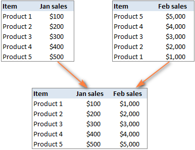
In this case, the Merge Two Tables add-in will work a treat:
- Select any cell in your main table and click the Merge Two Tables button on the Ablebits Data tab, in the Merge group:

This will run the add-in with your main table preselected, so in the first step of the wizard you simply click Next. - Select the second table, i.e. the lookup table containing the matching rows.

- Choose one or more column columns that exist in both tables. The key columns should contain only unique values, like Product ID in our example.

- Optionally, select the columns to update in the main table. In our case, there are no such columns, so we just click Next.
- Choose the columns to add to the main table, Feb sales in our case.

- In the final step, you can select additional options depending on how exactly you want to merge data, and click the Finish button. The screenshot below shows the default settings, that work just fine for us:

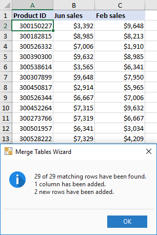
Allow the add-in a few seconds for processing and review the result:
How can I get these merging tools for Excel?
All of the add-ins discussed in this tutorial, plus 70+ other time-saving tools, are included in our Ultimate Suite for Excel. The add-ins work with all versions of Excel 2019, Excel 2016, Excel 2013, Excel 2010 and Excel 2007.
Hopefully, you can now merge rows in your Excel sheets exactly the way you want them. If you have not found a solution for your specific task, just leave a comment and we will try to figure out a way together. Thank you for reading!
Available downloads
Ultimate Suite 14-day fully-functional version (.exe file)
 by
by
118 comments
I have two rows of data with multiple columns. The data in row A has some of the same information in certain columns as in row B but there are blank columns in each where there is information in one but not the other column. I want to blend/merge all the columns into 1 row. The entire Excel has multiple sets of 2 rows that need to be done. I also have a column with different information in row A than in row B. I don't know of an easy way to put that one piece of data into a new column except to cut and paste.
Hello Dana!
Your question is not very clear because in Excel A and B are columns, not rows. If your phrase “merge all the columns into 1 row” means that you want to merge values from two columns, then try using this guide: How to merge two columns in Excel without losing data.
I recommend paying attention to Merge cells tool. It can combine columns and save the result to the left or to the right column. The tool is included in the Ultimate Suite for Excel and can be used in a free trial to see how it works.
If this is not what you wanted, describe the problem in more detail, provide me with an example of the source data and the expected result.
Hi, I bought Ablebits, and used it for a merge which worked great IF I had rows with a common column factor like email.
Here's the task I have now; it's an excel file exported out of Quickbooks.
It only lists client name ONCE, (and the columns are blank to the right), then BELOW, "blanks" in the name column, name is not repeated.
I want to end up with simply rows with "the client name", and the rows that had been below, "data from each row, each column", merged, in essence then having no blank rows. Purpose, so I can import into a CRM. Here's what the spreadsheet looks like:
NAME (blank) (blank)
(blank) [bought a house] [red]
(blank) [bought a plane] [blue]
Totals for NAME (blank) (Amount)
New NAME Then same pattern repeated
I need to merge, but since there is no data on the same row as NAME, then no repeating name in the rows below for "who it is", just data in the columns to the right... I'm having trouble seeing how to end up with simple rows, and "all data jammed into a cell" from the rows below the row which has the person's name (and that "all data merged" cell, ON the "name row", no blank rows... so it looks like a database in essence).
If you can visualize an accounting report from Quickbooks that has 'items bought" in columns (then a row showing the summary total), then a new name, well that is what this spreadsheet is. THE PATTERN IS NOT CONSISTENT, re: "how many rows are below a name", how many items purchased let's say.
I don't mind "all data in rows below the name row" being jammed together in one cell, as I'll be doing a keyword search function, it doesn't have to look nice.
But how do I accomplish this (again I have Ablebits), so it ends up like this:
Name1 [column with merge of the rows that had been below this name] [same, with rows merged]
Name2 [column with merge of the rows that had been below this name] [same, with rows merged]
Name3 [column with merge of the rows that had been below this name] [same, with rows merged]
Hello Frank! If I understand correctly, you need to fill the blank cells with the name that is written above in the column. To do this, use the Fill Blank Cells tool. Fill Blank Cells automatically fills the blank cells in a column with the value from the cell above or below it.
You can then merge rows with the same names in a column without losing information.
I hope it’ll be helpful. If something is still unclear, please feel free to ask.
THANK YOU Alexander!
That is Exactly what I needed, and it worked perfectly.
I had no idea there was a Fill Blank Cells tool.
Thanks for the Fast Help, you guys are great!
This tool was extremely easy to use and merged my list exactly how I needed it to be. Feels too good to be true, at a price of $0. Thank you Ablebits!
Hi, I have the following data, that I would like to merge, but sum up the quantity. I would really appreciate your help please.
Customer Project Name Reference Staff Quantity
Red Window A2163 John 0.5
Red Window A2163 John 0.5
Red Window A2163 John 3.75
Red Window A2163 Bruce 1
Red Window A2163 Bruce 2.25
Red Window A2163 James 3.75
Red Door A2174 Amy 1
Red Door A2174 Amy 0.75
Red Door A2174 Amy 2.25
Red Door A2174 Amy 0.5
Red Door A2174 Bruce 1.5
Red Door A2174 Bruce 2.25
Red Door A2174 James 3
Red Door A2174 James 6.25
Blue Window A3009 Bruce 2.25
Blue Window A3009 Bruce 3
Blue Window A3009 John 0.75
Blue Door A2946 Jane 4
Blue Door A2946 Jane 2.25
Blue Door A2946 Jane 1.75
Blue Door A2946 Amy 6
Just to clarify - If the customer, Project Name, Reference & staff are the same, then merge and total up the quantity.
So the duplicate lines, would merge, with the quantity added together, the desired result would be as follows:
Red Window A2163 John 4.75
Red Window A2163 Bruce 3.25
Red Window A2163 James 3.75
Red Door A2174 Amy 4.5
Red Door A2174 Bruce 3.75
Red Door A2174 James 9.25
Blue Window A3009 Bruce 5.25
Blue Window A3009 John 0.75
Blue Door A2946 Jane 8
Blue Door A2946 Amy 6
Hi! You can get the desired result in a couple of clicks without using formulas using Remove Duplicates tool. Specify that the duplicates are in the first four columns, and you want to summarise the fifth column. It is available as a part of our Ultimate Suite for Excel that you can install in a trial mode and check how it works for free.
Another way is to use subtotals in Excel. This article may be helpful: How to add, use and remove Subtotals in Excel.
In addition, you can use a pivot table to get totals for multiple metrics. Read more: How to make and use Pivot Table in Excel.
You can also calculate the sum of multiple criteria using the SUMIFS function. Look for the example formulas here: Excel SUMIFS and SUMIF with multiple criteria – formula examples.
I HAVE BELOW DATA ,NEED TO COMBINED IN ONE ROW
03-Nov-2023 DI048061 Hegde & Hegde Pharmaceutica LLP 27AAHFH3649H1Z7 27-MAHARASHTRA 998551 2,165.84 RP1L2F 65.75 18.00 0.00 5.92 5.92
03-Nov-2023 DI048062 Hegde & Hegde Pharmaceutica LLP 27AAHFH3649H1Z7 27-MAHARASHTRA 998551 3,557.24 MP42FV 134.70 18.00 0.00 12.12 12.12
03-Nov-2023 DI048063 Hegde & Hegde Pharmaceutica LLP 27AAHFH3649H1Z7 27-MAHARASHTRA 998551 18,193.08 2283543167878 108.75 18.00 0.00 9.79 9.79
2283543167879 108.75 18.00 0.00 9.79 9.79
2283543167880 108.75 18.00 0.00 9.79 9.79
2283543167881 98.75 18.00 0.00 8.89 8.89
2283543167882 98.75 18.00 0.00 8.89 8.89
2283543167883 98.75 18.00 0.00 8.89 8.89
Have you tried the methods described in this blog post? If you are not satisfied, please let me know and I will try to help you.
Goodday
question; i have an excel spreadsheet with daily sales of three mths and nine stores ,i will like to place this document into one sheet for nine stores so i can be able to see what what the stores sold by week.
Hi! Depending on what you want to do, there may be different answers. Try using a pivot table to show data for any store for any period of time. You can also use the FILTER function to get sales data by store for a week. To simply calculate the sum of sales for the week, you can use the SUMIFS function.
I have this date in excel sheet more then 300 entry, i want only column b date merge two row in one row, how to do this please any suggestion.
Date Particulars
-----------------------------------------------------
03/04/2023 Surplus Margin Received
from SMTF
05/04/2023 Cash Margin Transferred
to SMTF
06/04/2023 Money PayoutS
06/04/2023 Surplus Margin Received
from SMTF
10/04/2023 BG DP BILL AMOUNT DEBITE
D FOR DP ID 120333001009
6354
10/04/2023 Surplus Margin Received
from SMTF
11/04/2023 Cash Margin Transferred
to SMTF
12/04/2023 BEING DP BILL AMT RECD F
ROM BROKING FOR DP CLIEN
T CODE N10205593 & BROK
CODE 10910089
12/04/2023 Cash Margin Transferred
to SMTF
13/04/2023 BEING DP BILL AMT RECD F
ROM BROKING FOR DP CLIEN
T CODE N10205593 & BROK
CODE 10910089
Hi! Have you tried the ways described in this blog post? If they don’t work for you, then please describe your task in detail, give an example of the desired result.
I have below data (Data Source) in sheet1.
C D E F G H I J
1 Depart Arrive Depart Arrive Airline Airline Total Duration Stopover
2 10:00 (BOM) 18:10 (DEL) 12:20 (DEL) + 1 05:30 (ICN) ABC AIR (AB 909) A2Z Air (2Z 668) 16h DEL5h 50m
3 11:45 (BOM) 23:00 (SIN) 19:50 (SIN) + 1 06:20 (ICN) RST Air (ST 406) A2Z AIR (2Z 752) 15h 05m SIN3h 10m
4 13:15 (BOM) 23:20 (KUL) 21:05 (KUL) + 1 06:50 (ICN) MNO Air (MO 275) KLN AIR (KN 672) 14h 05m KUL2h 15m
5 13:15 (BOM) 23:30 (KUL) 21:05 (KUL) + 1 07:10 (ICN) MNO Air (MO 275) MNO Air (MH 66) 14h 25m KUL2h 25m
In Sheet2 i have extracted data from Data Source File as below
A B C D E F G H I
1 Flt No Days of Ops FPW From To Dep Arr Transit Flying Time
2 AB 909 M-W-F-- 3 BOM DEL 10:00 12:20 5h 50m 16h
3 2Z 668 DEL ICN 18:10 05:30
Here's how i have extracted the data in sheet2
Column A Formula: MlD(Sheet1!G2,SEARCH("(",Sheet1!G2)+1,SEARCH(")",Sheet1!G2,SEARCH(",Sheet1!G2)+1)-SEARCH("(",Sheet1!G2)-1)
Column B Formula: =CONCATENATE(Sheet1!L2,Sheet1!M2,Sheet1!N2,Sheet1!O2,Sheet1!P2,Sheet1!Q2,Sheet1!R2,)
Column C Formula: =Sheet1!S2
Column D Formula =MlD(Sheet1!C2,8,3)
Column E Formula =MlD(Sheet1!E2,8,3)
Column F Formula: =LEFT(Sheet1!C2,5)
Column G Formula: =LEFT(Sheet1!E2,5)
Column H Formula: =RlGHT(Sheet1!J2,6)
Column I Formula: =RlGHT(Sheet1!I2,6)
My question is when i copy formula from 2nd and 3rd row in output file and paste in fourth row it gives result of 4th row data of data file i.e shhet1.
But I need the data of 3rd row of Data file i.e sheet1.
Is it possible to achieve this.
Regards/Irfan
Hi! Copying a formula changes the relative row and column references. I recommend reading this manual: Relative and absolute cell reference: why use $ in Excel formula.
Thanks Alexander for your reply
Kindly give me an example how to use reference in this case.
Again i would like to clarify when i copy formula from 2nd and 3rd row in sheet2 and paste in fourth and fifth row it gives result of 4th row data of data file i.e sheet1.
But I need the data of 3rd row of Data file i.e sheet1. (When I copy 2 & 3 row and paste in 4 & 5 row row reference should move only 1 row instead of two)
for your reference data as below for your understanding
I have below data (Data Source) in sheet1.
C | D | E | F | G | H | I | J
1 | Depart | Arrive | Depart | Arrive | Airline | Airline | Total Duration | Stop Over
2 | 10:00 (BOM) | 18:10 (DEL) |12:20 (DEL) + 1 | 05:30 (ICN) | ABC AIR (AB 909) |A2Z Air (2Z 668) | 16h | DEL5h 50m
3 |11:45 (BOM) | 23:00 (SIN) | 19:50 (SIN) + 1 | 06:20 (ICN) | RST Air (ST 406) | A2Z AIR (2Z 752) | 15h 05m | SIN3h 10m
4 | 13:15 (BOM) | 23:20 (KUL) | 21:05 (KUL) + 1 | 06:50 (ICN) | MNO Air (MO 275) | KLN AIR (KN 672) | 14h 05m | KUL2h 15m
5 | 13:15 (BOM) | 23:30 (KUL) |21:05 (KUL) + 1 | 07:10 (ICN) | MNO Air (MO 275) | MNO Air (MH 66) | 14h 25m | KUL2h 25m
In Sheet2 i have extracted data from Data Source File as below
A | B | C | D | E | F | G | H | I
1 | Flt No | Days of Ops | FPW | From | To | Dep | Arr | Transit | Flying Time
2 | AB 909 | M-W-F-- | 3 | BOM | DEL | 10:00 | 12:20 | 5h 50m | 16h
3 | 2Z 668 | | | DEL | ICN | 18:10 | 05:30
Here's how i have extracted the data in sheet2
Column A Formula: MlD(Sheet1!G2,SEARCH("(",Sheet1!G2)+1,SEARCH(")",Sheet1!G2,SEARCH(",Sheet1!G2)+1)-SEARCH("(",Sheet1!G2)-1)
Column B Formula: =CONCATENATE(Sheet1!L2,Sheet1!M2,Sheet1!N2,Sheet1!O2,Sheet1!P2,Sheet1!Q2,Sheet1!R2,)
Column C Formula: =Sheet1!S2
Column D Formula =MlD(Sheet1!C2,8,3)
Column E Formula =MlD(Sheet1!E2,8,3)
Column F Formula: =LEFT(Sheet1!C2,5)
Column G Formula: =LEFT(Sheet1!E2,5)
Column H Formula: =RlGHT(Sheet1!J2,6)
Column I Formula: =RlGHT(Sheet1!I2,6)
Hi! If you copy a formula from row 2 to row 4, it will reference row 4, not row 3 as you want. This is how copying works in Excel.
I have the following group of data in excel:
Location
ID
Name
Grade
Subject
Cred Term
Doc #
Eff Beg
Eff end
Some ID's have multiple lines as they have multiple certifications. I would like to merge all certifications into one line by ID.
I currently have Ablebits software.
Hi!
Use Ablebits Data - Merge Duplicates.
Step 1. Select your table.
Step 2. Choose key columns - select ID column
Step 3. Choose columns with the values to merge - select all other cloumns or only some of the columns whose data needs to be merged
You can also read the detailed instructions for the Merge Duplicates tool here: How to combine duplicate rows in Excel.
I hope I answered your question. If something is still unclear, please feel free to ask.
Hi!! Thank you for helping people find solutions! How do I merge duplicate rows (of customers) info into one row with the customers info in multiple columns?
Like Customer one came into the store on dates (data in each row in separate columns) so each customer only has 1 row instead of 5 rows.
My end goal is to have Customer 1 in one row with all of their visit dates in one row. Right now, there Visit dates are on their own row (but in different columns).
Thx!!
Kelley
Hello!
I recommend that you use the Merge Duplicates tool. You can quickly combine duplicate rows into one without losing any data. It is available as a part of our Ultimate Suite for Excel that you can install in a trial mode and check how it works for free.
A B C
Sr Container
1 MSKU123456
TCLU123456
2 TCLU123456
3 PONU123456
MIEU123456
MRSU123456
MRSU123456
This is the list of my data i want to merge my container No in Coumn C but Rowas are not Fixed
Sorry, I do not fully understand the task.
As it's currently written, it's hard to tell exactly what you're asking.
Hi,
I have an excel sheet data dump available where there is following information :-
Column A - Name of Organization
Column B - License
Column C - Address
In some cases, the address in column C is in one row and in some cases multiple rows (for example, 4 or 5). And when address is in multiple rows, the name of the organization and license has been merged, meaning,
Column A
Cells A1 to A4 are merged
Column B
Cells B1 to B4 are merged
Column C
C1 - 1st line of address,
C2 - 2nd line of address
C3 - 3rd line...
C4 - 4th line of address.
Now manually using the merge cell by row helps with individually merging C1 to C4 cells. However, is there a way I can apply that logic on the entire excel sheet in one attempt ? Thank you for your help.
Regards,
Jai
Hello!
Merge cells D1:D4. You can use Excel's Merge & Center feature. Then write the formula =CONCATENATE(C1,C2,C4,C4) in that cell. After that you can copy this formula down along the column.
This should solve your task.
Hi. re: "How to combine duplicate rows into one (keeping unique values only)" section of this article, does Ablebits have a tool that will do the inverse/opposite of this? i.e. delimit the merged values and repeat/duplicate the respective key column value for each of the delimited values?
To elaborate a little more, what I am trying to achieve is similar to what is described here:
http s://stackoverflow.com/questions/44655553/vba-excel-with-thousands-of-rows-how-to-transpose-variable-length-columns-to
But instead of a macro, I am wondering if Ablebits offers a tool that does the same?
Hello!
We have a tool that can solve your task in a couple of clicks - first you use the tool Merge Cells - Merge Columns Into One. You are merge the Property1-Property6 values in one column by separating them with a semicolon, for example. Then you use Split Text - Split by Characters - Split to Rows and get the desired result.
It is available as a part of our Ultimate Suite for Excel that you can install in a trial mode and check how it works for free.
Hello!
You can get all the unique values in one cell using the Duplicate Remover - Uniques and 1st Occurrences tools.
You can split these values into cells using the Split Text tool.
However, Ultimate Suite cannot restore the previous number of duplicates and return data to its original state.
You can install Ultimate Suite for Excel in a trial mode and check how it works for free.
W/O COUSTOMER NAME Colour Count
01/21 SMART LUNGI GREEN 80/2CD
01/21 SMART LUNGI YELLOW 80/2CD
02/21 T.T.I TEXTILE WHITE 20/1CD
03/21 URMI WEAVING A-109 50/1CTN
03/21 URMI WEAVING A-151 40/1VISCOSE
04/21 MOMTEX EXPO WHITE 10/1CD
04/21 MOMTEX EXPO WHITE 16/1CD
I need when i write 01 then auto color (green & yellow) show in specific 2 raws like
01/21 = green yellow or data validation list wise show green and yellow, It depends when i input the data in selected raw then that result show other coloums raws
Hi!
If I understand the problem correctly, use the IF function to assign a color based on the number in the cell.
If I am not guessing, please explain your question in more detail.
Hello,
I have a data set where each item has several duplicates. I need to get rid of the duplicates while summing an amount in each duplicate to get a total for each set of duplicates.
Hello, I have a master spreadsheet and receive a daily updated spreadsheet, both are sorted alpha by name, and each row of names has several columns with data specific to that name (i.e. address/phone #). The master sheet has two additional columns with data entered only on the master. The daily sheet contains new names that are not contained in the master, as well as the names that are in the master. I would like to merge the two spreadsheets without duplicating names, and only bringing in the new names and the data that is contained in all columns of the new names without losing the additional columns/data that are only in the master.
Hello!
Unfortunately, without seeing your data it hard to give you advice.
I'd recommend you to have a look at our Ablebits Data- Merge Two Tables.
This tool is available as a part of our Ultimate Suite for Excel that you can install in a trial mode and use for 30 days for free: https://www.ablebits.com/files/get.php?addin=xl-suite&f=free-trial
Hello,
if i have data in multiple row and a few data are in common, I can I merge the rows?
Example:
Column A / Column B / Column C
Row 1. Name1 / Phone1 / Nothing
Row 2. Name2 / Phone2 / Company2.a
Row 3. Nothing / Phone1 / Company1
Row 4. Name2 / Nothing / Company2.b
The result that i want is:
Column A / Column B / Column C
Row 1. Name1 / Phone1 / Company1
Row 2. Name2 / Phone2 / Company2.a, Company2.b
Is it possible?
Thank you
that right there is exactly what i need!
Hello I have a spreadsheet with the following info:
Name City Store 1 Store 2 Store 3
John New York Missing sign No issue Missing paper
Mary Chicago No issue Missing Light No issue
Sam Atlanta Missing paper Missing carpet Missing paper
I have to generate a report that looks like this:
Name City Location Issue
John New York Store 1 Missing Sign
John New York Store 3 Missing paper
Mary Chicago Store 2 Missing light
Sam Atlanta Store 1 Missing paper
Sam Atlanta Store 2 Missing carpet
Sam Atlanta Store 3 Missing paper
Any suggestions would be greatly appreciated!
Thank you
I am trying to merge all the rows into one ,but i am still losing a lot of values,is their a limit to the tool.
Supposing you have a range of data as below screenshot shown. Now you may need to merge rows of data with the same value in the Fruit column. In this condition, you can apply the Advanced Combine Rows feature of Kutools for Excel to deal with it.