In this short tutorial, you will find many helpful details about Excel percent format and learn how to format existing values as per cents, how to show percentage in empty cell and change numbers to percentages as you type.
In Microsoft Excel, displaying values as percentages is very straightforward. To apply the percent format to a given cell or several cells, select them all, and then click the Percent Style button in the Number group on the Home tab:
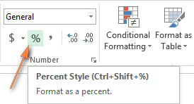
Even a faster way is pressing the Ctrl + Shift + % shortcut (Excel will remind you of it every time you hover over the Percent Style button).
Although formatting numbers as percentages in Excel takes just a single mouse click, the results may vary depending on whether you apply the percent formatting to existing numbers or empty cells.
Formatting existing values as percentage
When you apply the Percentage format to cells that already contain numbers, Excel multiplies those numbers by 100 and adds the per cent sign (%) at the end. From Excel's viewpoint, this is the correct approach since 1% is one part of one hundred.
However, this way does not always work right. For example, if you have 20 in cell A1 and you apply the percentage format to it, you will get 2000% as the result, and not 20% as you might expect.
Possible workarounds:
- Calculate numbers as percentages before applying the percent format. For example, if your original numbers are in column A, you can enter the formula
=A2/100in cell B2 and then copy it down to all other cells in column B. Then select the entire column B and click the Percent Style. You will get a result similar to this:
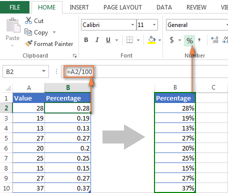
Finally, you can replace the formulas with values in column B, copy them back to column A and delete column B if you do not need it any longer.
- If you want to apply the percentage formatting to just a few numbers, you can type a number in its decimal form directly into the cell. For example, to have 28% in cell A2, type 0.28 and then apply the percentage format.
Applying percentage format to empty cells
Microsoft Excel behaves differently when you enter numbers into empty cells pre-formatted as Percentage:
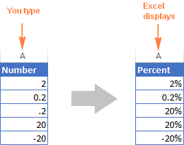
- Any number equal to or greater than 1 is converted to a percent by default. For example, 2 is turned into 2%, 20 into 20%, 2.1. into 2.1% and so on.
- Numbers smaller than 1 without a preceding zero are multiplied by 100. For example, if you type .2 in a percentage preformatted cell, you'll see 20% in that cell. However, if you enter 0.2 in the same cell, 0.2% will appear exactly as it should.
Display numbers as percentages as you type
If you type 20% (with the percentage sign) directly in a cell, Excel will understand that you are entering a percent and will apply percentage formatting automatically.
Important note!
When applying the percentage formatting it Excel, please keep in mind that it is nothing more but a visual representation of a real value stored in a cell. The underlying value is always stored in decimal form.
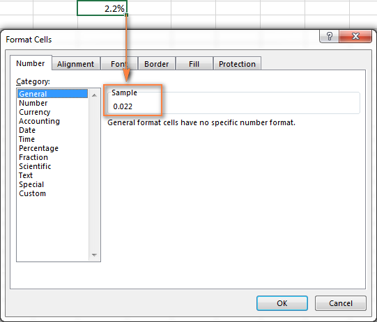
In other words, 20% is stored as 0.2, 2% is stored as 0.02, 0.2% is 0.002, etc. When performing calculations, Excel always deals with the underling decimal values. Please remember this fact when referencing percent cells in your formulas.
To see the real value behind percentage formatting, right-click the cell, click Format Cells (or press Ctrl + 1) and look in the Sample box under the General category on the Number tab.
Tips to display percentages in Excel
Showing percentage in Excel seems to be one of the earliest tasks, right? But experienced Excel users know that a path to the goal almost never runs smooth :)
1. Display as many decimal places as you want
When applying the percent formatting to numbers, Excel sometimes shows rounded percentages with no decimal places, which may cause some confusion. For example, apply the percent format to an empty cell and then type 0.2 into it. What do you see? In my Excel 2013, I see 0% though I know with certainty it should be 0.2%.
To see the actual percentage instead of a rounded version, you just need to increase the number of decimal places showing. To do this, open the Format Cells dialog either by pressing Ctrl + 1 or right-clicking the cell and selecting Format Cells… from the context menu. Make sure the Percentage category is selected and specify the desired number of decimal places in the Decimal places box.
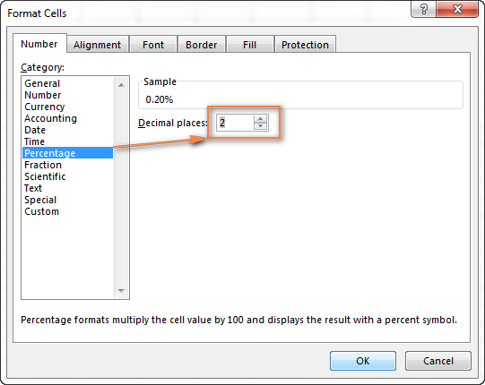
When done, click the OK button to save your settings.
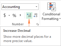
Alternatively, you can control the number of displayed decimal places, by clicking the Increase Decimal or Decrease Decimal icons on the ribbon (Home tab > Number group):
2. Apply a custom format to negative percentages
If you want to format negative percentages in a different way, say in red font, you can create a custom number format. Open the Format Cells dialog again, navigate to the Number tab > Custom category and enter one of the below formats in the Type box:
- 00%;[Red]-0.00% - format negative percentages in red and display 2 decimal places.
- 0%;[Red]-0% - format negative percentages in red without any decimal places showing.
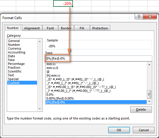
You can find more details about this formatting technique in the Display numbers as percentages article by Microsoft.
3. Format negative percentages using Excel conditional formatting
Compared to the previous method, Excel conditional formatting is more versatile and it lets you display negative percentages, e.g. percent decrease, in any format of your choosing.
The fastest way to create a conditional formatting rule for negative percentages is to click Conditional formatting > Highlight cells rules > Less than and put 0 in the "Format cells that are LESS THAN" box:
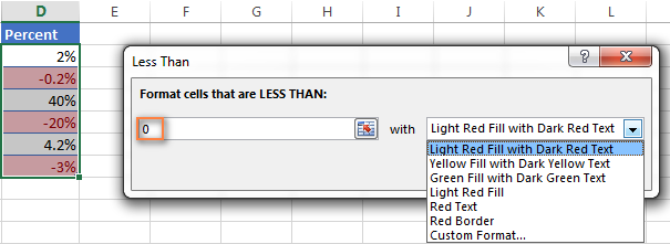
Then you choose one of the formatting options from the drop-down list on the right, or click Custom Format... at the end of the list to set up for own formatting.
For more information about creating conditional formatting rules, please see How to use conditional formatting in Excel.
This is how you work with Excel percent format. Hopefully, this knowledge will help you avoid a lot of headache when you in the future. In the next articles, we are going to learn how to calculate percentages in Excel and write formulas for percent change, percentage of a total, compound interest and more. Please stay tuned and thank you for reading!
 by
by
42 comments
I have 7 rows with a dollar amount of doctors' production of goods. I need to get a % of all those at the ends. How do I figure that out on a worksheet?
Hi!
Maybe this article will be helpful: How to calculate percentage in Excel - formula examples.
If I have two totals and I want to shoe the %. Example Total is 60, but only 43 are good. need to figure the 5 of good out of the total.
Thanks
Hi!
Sorry, it's not quite clear what you are trying to achieve.
How would i input the formula to calculate the following;
Collumns E, F & G - how would i show in G the percentage in F of the amount in E so for example;
E = 1000
F = 5%
G = This should show up as 50
There will always be amounts in columns E & F
Hi!
How to multiply a number by a percentage - read this article: How to calculate percentage in Excel – percent formula examples.
Can someone help me please
I’m trying to calculate x as a percentage of sales.
E.g
Sales are 2,000,000.00
COG are 25%
I want to show the financial (500k) as a number not as a percentage
Hello!
If I understand your task correctly, use the formula
=A1 * 25%
or =A1 * 0.25
Set the cell to a number format as described in this article.
Hi I need to calculate percentages by occupancies
so if I have 5 people and I have 20 spots, the percentage should 25%, I want to know if there is any simple way to apply a formula here as it is taking me so much time thank you.
Hi
I need to work out a percentage on KPI measures in our reponse time
Let say: We had on incident at a area response time are 5min but we respond within 7min so how will I work out my incident response time for VDC for the month
Let say:We had total of 23 incidents for the month only 22 incidents were within the response time and 1 was not with in. How do I work out my response KPI
If I insert =4/20 the result will display .20 which is correct but if I insert =(22-20)+2/20 the result is .21 which is incorrect. How do I get excel to display the correct answer in to =(22-20)+2/20?
Hello!
When I write in the cell Excel =(22-20)+2/20, I get the result 2.1
Perhaps your .21 result is due to the number set in the custom format cell.
Sir,
10% =right(j10,1)
not show ( % percent sign)
$20.00- $18.00 = $2.00/20 * 100 % =10 %. thus you give him a discount of 10%
Dear Madam/Sir
Good Evening,
Greetings!
I need help
I gave the price to the customer 20.00$ and he gave me offer 18.00$ (how much percentage he reduce the prices?
total class 4
one student present in class 4
how to use presentage ratio 100
send me presentage formula
I have a a document showing whether someone was late, early or on time. I need to get the percentage of how any times someone was late, early or on time. The thing is, is that it's marked down as "X" in the appropriate column and I don't know how to get the percentage. Help, please?!
How can I find the 20 % mark of a students mark, I want to prepare progress report. I just want to know the formula.
If I am trying to calculate room occupancy with time how to do it. for example,
There are a total of 40 hours the class can be used per week from 8-4.
Classes are
8:00 am to 10:40 am 2 classes per week at 5.20 hours
9:30 am to 10:45 am 2 classes per week at 2.30 hours
How do I find the percentage of time used of the classroom. If there are 40 total hours the class can be used and one class is at 5.20 hours of usage per week and another is 2.30 hours per week - what is the percentage of use time for each individual class out of 40 hours.
Thanks,
Audrey
F2 value 69050 how to calcutae 20%
Price AMC
69050 calculate for this AMC
69050
69050
69050
I am trying to deduct a percentage (%) from a cell into another cel?
A B C D E F G H I J
1. Model Outlet 2019 LIST -25% -30% -33% -35% -37% -40%
2.LB-480 2" 575.00
3.
For example i want to have E3 to show D9-25%
Can anyone help Please!
Trying to learn how to use excel better at work I need to try and find the percentage of staff who have completed training so let's say 30 staff and in the B column are all the dates I.e. 23/09/2017 how do I work out the percentage of the number of staff with dates next to there names. Then could I put the total percentage onto a different page. Can anyone help
I have values in my excel in columns as
48GB 78GB 21GB
3.9TB 5.3TB 9.2TB
where GB is Gigabytes and TB is terrabytes I have to calculate percentages of above data but due to GB and TB in numbers I am getting errors. How can this be sorted out.
I think there are at least two ways to solve your problem.
If you don't have many of these rows to split, just use the Text-to-Columns tool in Excel. Under Data choose the Text-to-Columns use the fixed width and that should do it. What I did when I was practicing with your sample data was to copy and Paste Special/Transpose it so I could get it into columns so I could split the top three into columns and then the second three.
If you have a lot of this data you can use this formula. It will split out the numbers for you. It needs to be entered with CTRL+Shift+Enter because it is an array. You can change E9 to the address you need.
=LOOKUP(10^99,--MID("|"&E9,SMALL(IF(((--ISNUMBER(--MID("|"&E9, ROW($1:$1003),1))=0)*ISNUMBER(--MID("|"&E9,ROW($2:$1004),1))),ROW($2:$1004)),1), ROW($1:$1003)))
Can you please help me get notes and examples of using the financial functions in excel.
Let me thank you very much for the excel knowledge you are sharing. Please keep it up and know that we are very grateful.
1099
494
i want find percentage of few values
books 20
paper 30
table 100
chairs 20
total 170
how can i find the percentage.