This page can be your entry point to learning Microsoft Excel functions. It lists the most essential text, math, statistical, logical and other functions along with formula examples and links to related resources.
Excel provides an enormous number of functions to analyze, audit and calculate data. Some of them are utilized by many Excel users on a daily basis while others are so very specific that only a small group of financial, statistical or engineering specialists understand and need them.
In this tutorial, we do not aim to explorer all and each function available in Microsoft Excel. On this page, you will find the most useful and most used Excel functions, which we've already covered in depth in individual step-by-step guides.
Most of the functions listed below are Excel worksheet functions that are used as part of formulas in a cell. The last category includes custom Excel functions, aka user-defined functions (UDF). These are VBA-based functions that extend the basics of Excel with custom functionality. Select a category to go to the functions list with short descriptions and links to examples of use.
Excel text functions (string functions)
There exist a great lot of Microsoft Excel functions to manipulate text strings. Here are the most essential ones:
TEXT function
TEXT(value, format_text) is used to convert a number or a date into a test string in the specified format, where:
- Value is a numeric value you want to convert to text.
- Format_text is the desired format.
The following formulas demonstrate the Excel TEXT function in action:
=TEXT(A1,"mm/dd/yyyy") - convert a date in cell A1 into a text string in the traditional US date format, such as "01/01/2015" (month/day/year).
=TEXT(A1,"€#,##0.00") - converts a number in A1 into a currency text string such as "€3.00".

TEXT formula examples:
CONCATENATE function
CONCATENATE(text1, [text2], …) is designed to join several pieces of text together or combine values from several cells into a single cell. An analogues result can be achieved by using the Excel & operator, as demonstrated in the following screenshot.

You can find plenty more formula examples in the tutorial CONCATENATE in Excel: combine text strings, cells and columns.
TRIM function
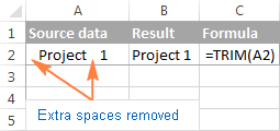
TRIM(text) removes leading, trailing spaces as well as excess spaces between words. Where text is either a text string or reference to the cell containing the text from which you want to remove spaces. The following screenshot demonstrates an example of usage:

For more formula examples, see 3 ways to remove spaces between words / numbers in Excel.
SUBSTITUTE function
SUBSTITUTE(text, old_text, new_text, [instance_num]) replaces one set of characters with another in a specified cell or a text string. The syntax of the SUBSTITUTE function is as follows:
- Text - the original text string or reference to a cell where you want to substitute certain characters.
- Old_text - the characters you want to replace.
- New_text - the characters you want to replace the old text with.
- Nth_appearance - an optional parameter that specifies which occurrence of old_text you want to replace with new_text. If omitted, then every occurrence of the old text will be replaced with the new text.
For example, the following SUBSTITUTE formula replaces all commas in cell A1 with semicolons:
=SUBSTITUTE(A2, ",", ";")

SUBSTITUTE formula examples:
VALUE function
VALUE(text) - converts a text string to a number.
This function is really helpful when it comes to converting text-formatted values representing the numbers into numbers that can be used in other Excel formulas and calculations.
VALUE formula examples:
EXACT function
EXACT(text1, text2) compares two text strings and returns TRUE if both values are exactly the same, including case, FALSE otherwise.
For example, if A2 is "apples" and B2 is "Apples", the formula =EXACT(A2, B2) will returns FALSE, because they are not exact match.
The EXACT function is rarely used on its own, but it's helpful in more complex tasks such as doing a case-sensitive Vlookup in Excel.
Functions to change text's case (UPPER, LOWER, PROPER)
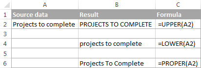
Microsoft Excel provides 3 text functions to convert between UPPER, lower and Proper case.
UPPER(text) - converts all characters in a specified text string to upper case.
LOWER(text) - changes all uppercase letters in a text string to lowercase.
Proper(text) - capitalizes the first letter of each word and converts all other letters to lowercase (more precisely, it capitalizes the letters that follow any character other than a letter).
In all three functions, the text argument can be a text string enclosed in quotation marks, a reference to a cell containing the text or a formula that returns the text.

More formula examples to convert text's case can be found in Changing text case in Excel to UPPER, lower or Proper.
Extract text characters (LEFT, RIGHT, MID)
If you need a formula to return a certain number of characters from a text string, use one of the following Excel functions.
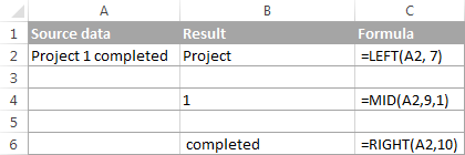
LEFT(text, [num_chars]) - returns a specified number of characters from the beginning of a text string.
RIGHT(text,[num_chars]) - returns a specified number of characters from the end of a text string.
MID(text, start_num, num_chars) - returns a specific number of characters from a text string, starting at any position that you specify.
In these functions, you supply the following arguments:
- Text - a text string or a reference to a cell containing the characters you want to extract.
- Start_num - indicates where to start (i.e. the position of the first character you want to extract).
- Num_chars - the number of characters you want to extract.

One of the main uses of these Excel text functions is splitting a cell's content into several cells, as demonstrated in Formulas to split cells in Excel.
Logical functions in Excel
Microsoft Excel provides a handful of logical functions that evaluate a specified condition(s) and return the corresponding value.
AND, OR, XOR functions
AND(logical1, [logical2], …) - returns TRUE if all of the arguments evaluate to TRUE, FALSE otherwise.
OR(logical1, [logical2], …) - returns TRUE if at least one of the arguments is TRUE.
XOR(logical1, [logical2],…) - returns a logical Exclusive Or of all arguments. This function was introduced in Excel 2013 and is not available in earlier versions.

Logical functions formula examples:
NOT function
NOT(logical) - reverses a value of its argument, i.e. if logical evaluates to FALSE, the NOT function returns TRUE and vice versa.
For instance, both of the following formulas will return FALSE:
=NOT(TRUE)
=NOT(2*2=4)
For more NOT function examples, see Using the NOT function in Excel.
IF function
The Excel IF function is sometimes called a "conditional function" because it returns a value based on the condition that you specify. IF's syntax is as follows:
An IF formula tests the condition(s) expressed in the logical_test argument and returns one value (value_if_true) if the condition is met and another value (value_if_false) if the condition is not met.
For example, the formula =IF(A1<>"", "good", "bad") returns "good" if there's any value in cell A1, "bad" otherwise.
And here's an example of the nested IF formula that "deciphers" the exam score in cell A2:
=IF(A2>80, "Brilliant", IF(A2>50, "Good", IF(A2>30, "Fair", "Poor")))

IF formula examples:
IFERROR and IFNA functions
Both functions are used to check if a certain formula evaluates to an error, and if it does, the MS Excel functions return a specified value instead.
IFERROR(value, value_if_error) - checks if the formula or expression evaluates to an error. If it does, the formula returns the value supplied in the value_if_error argument, otherwise, the result of the formula is returned. This function handles all possible Excel errors, including VALUE, N/A, NAME, REF, NUM, and others. It is available in Excel 2007 and higher.
IFNA(value, value_if_na) - introduced in Excel 2013, it works similarly to IFERROR, but handles #N/A errors only.
The following examples demonstrate the simplest IFERROR formula:

IFERROR / IFNA formula examples:
Excel math functions
Excel has a ton of basic and advanced functions to perform mathematical operations, calculate exponentials, logarithms, factorials and the like. It would take several pages just to publish the functions list. So, let us discuss only a few basic math functions that may prove useful for solving your daily tasks.
Finding the sum of cells
Four essential Excel functions to add up the values of cells in a specified range follow below.
SUM function
SUM(number1,[number2],…) returns the sum of its arguments. The arguments can be numbers, cells references or formula-driven numeric values.
For example, the simplest math formula =SUM(A1:A3, 1) adds up the values in cells A1, A2 and A3, and then adds 1 to the result.
SUM formula examples:
SUMIF and SUMIFS functions (conditional sum)
Both functions add up the cells in a specified range that meet a certain condition. The difference is that SUMIF can evaluate only a single criteria, while SUMIFS, introduced in Excel 2007, allows for multiple criteria. Please pay attention that the order of arguments is different in each function:
- range / criteria_range - the range of cells to be evaluated by the corresponding criteria.
- criteria - the condition that must be met.
- sum_range - the cells to sum if the condition is met.
The following screenshot gives an idea of how the SUMIF and SUMIFS functions can be used on real-life data:

SUMIF and SUMIFS formula examples:
SUMPRODUCT function
SUMPRODUCT(array1,array2, …) is one of the few Microsoft Excel functions that handle arrays. It multiplies the supplied array components and returns the sum of the products.
The essence of the SUMPRODUCT function may be difficult to grasp, and hopefully the following examples will shed some light on its major uses.
SUMPRODUCT formula examples:
Generating random numbers (RAND and RANDBETWEEN)
Microsoft Excel provides 2 functions to generate random numbers. Both are volatile functions, meaning that a new number is returned every time the worksheet calculate s.
RAND() - returns a random real (decimal) number between 0 and 1.
RANDBETWEEN(bottom, top) - returns a random integer between the bottom and top numbers that you specify.
The following tutorial makes a pretty good job explaining the nuts and bolts of each function with formula examples: How to use RAND and RANDBETWEEN functions in Excel.
Rounding functions
There exist a variety of functions to round off numbers in Excel, and our Excel Rounding Tutorial makes a good job explaining how to use those functions based on your criteria. Please click on the function's name to learn its syntax and examples of uses.
- ROUND - round the number to the specified number of digits.
- ROUNDUP - round the number upward to the specified number of digits.
- ROUNDDOWN - round the number downward to the specified number of digits.
- MROUND - rounds the number upward or downward to the specified multiple.
- FLOOR - round the number down to the specified multiple.
- CEILING - round the number up to the specified multiple.
- INT - round the number down to the nearest integer.
- TRUNC - truncate the number to a specified number of decimal places.
- EVEN - round the number up to the nearest even integer.
- ODD - round the number up to the nearest odd integer.
Getting the remainder after division (MOD function)
MOD(number, divisor) returns the remainder after the number argument is divided by divisor.
The function comes in really handy in many scenarios, for example:
Statistical functions in Excel
Among a variety of highly specific Excel statistical functions, there are a few ones that everyone can understand and leverage for professional data analysis.
Finding the largest, smallest and average values
MIN(number1, [number2], …) - returns the minimal value from the list of arguments.
MAX(number1, [number2], …) - returns the maximum value from the list of arguments
AVERAGE(number1, [number2], …) - returns the average of the arguments.
SMALL(array, k) - returns the k-th smallest value in the array.
LARGE(array, k) - returns the k-th largest value in the array.
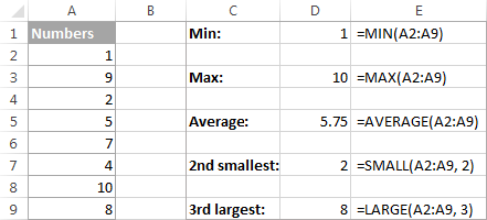
The following screenshot demonstrates the basic statistical functions in action.

Formula examples:
- Using IF with AVERAGE, MIN and MAX functions
- Calculating the average of the top N items in the list - Example 1. Calculate average of the top N items in the list
- VLOOKUP with AVERAGE, MAX, MIN (array formulas)
- Sum N largest / smallest numbers in a range (array formula)
Counting cells
Below is a list of Excel functions that let you count the cells containing a certain data type or based on the condition(s) that you specify.
COUNT(value1, [value2], …) - returns the number of numerical values (numbers and dates) in the list of arguments.
COUNTA(value1, [value2], …) - returns the number of non-empty cells in the list of arguments. It counts cells containing any information, including error values and empty text strings ("") returned by other formulas.
COUNTBLANK(range) - counts the number of empty cells in a specified range. Cells with empty text strings ("") are also counted as blank cells.
COUNTIF(range, criteria) - counts the number of cells within the range that meet the specified criteria.
COUNTIFS(criteria_range1, criteria1, [criteria_range2, criteria2]…) - counts the number of cells that meet all of the specified criteria.
The following screenshot demonstrates the counting cells functions in action:

Note. Since dates are stores as numbers in Excel, they are also counted by Excel statistical functions. For example, the formula =COUNTIF(A2:A9, ">5") counts the date in cell A8 in the screenshot above because it is stored as 42005 in the internal Excel system.
Counting cells formula examples:
Excel lookup and reference functions
These MS Excel functions comes in handy when you need to find certain information in a table based on a value in one column, or return a reference to a certain cell.
VLOOKUP function
The VLOOKUP function looks for a specified value in the first column and pulls the matching data from the same row in another column. It requires the following arguments:
- lookup_value - the value to search for.
- table_array - two or more columns of data.
- col_index_num - the number of the column to pull the data from.
- range_lookup - determines whether to search with exact match (FALSE) or approximate match (TRUE or omitted).
For example, the formula =VLOOKUP("apples", A2:C10, 3) searches for "apples" in cells A2 through A10 and returns a matching value from column C:
VLOOKUP formula examples:
INDEX function
INDEX(array, row_num, [column_num]) - returns a reference to a cell within array based on the row and column numbers that you specify.
Here is a simple INDEX formula: =INDEX(A1:C10, 3 ,4) that searches in cells A1 through C10 and returns a value at the intersection of the 3rd row and 4th column, which is cell D3.
The following tutorial explains the INDEX function in full detail: 6 most efficient uses of the INDEX function in Excel.
MATCH function
MATCH(lookup_value, lookup_array, [match_type]) - searches for lookup_value in lookup_array, and then returns the relative position of that item in the range.
The combination of the MATCH and INDEX functions can be used as a more powerful and versatile alternative to Excel's VLOOKUP, as demonstrated in the following tutorial: INDEX & MATCH - a better alternative to VLOOKUP in Excel.
INDIRECT function
INDIRECT(ref_text, [a1]) - returns a cell or range reference specified by a text string.
Here's an example of the simplest INDIRECT formula to get the general idea:

In real worksheets, INDIRECT formulas are often used to dynamically refer to another sheet or workbook, to lock a cell reference or to create dependent drop down lists.
INDIRECT formula examples:
OFFSET function
OFFSET(reference, rows, cols, [height], [width]) - returns a reference to a range of cells that is offset from a starting cell or a range of cells by the specified number of rows and columns.
For example, =OFFSET(A1, 1, 2) returns the value in cell C2 because it's 1 row down and 2 columns to the left from A1.
For more OFFSET formula examples, please see: Using OFFSET function in Excel.
TRANSPOSE function
TRANSPOSE(array) - transforms a horizontal range of cells into a vertical range and vice versa, i.e. converts rows to columns and columns to rows.
The following tutorial provides formula examples and explains the strong and weak points of the function: Excel TRANSPOSE function to convert row to column.
HYPERLINK function
HYPERLINK(link_location, [friendly_name]) - Creates a hyperlink to a document stored on a local network or the Internet.
For the step-by-step guidance in using the HYPERLINK function, please see: How to add a hyperlink to another Excel sheet.
Excel financial functions
Microsoft Excel provides a host of functions to simplify the work of accounting managers, financial analysts and banking specialists. On this blog, we have discussed only one financial function so far, which can be used to calculate compound interest.
FV function
FV(rate, nper ,pmt ,[pv], [type]) - calculates the future value of an investment based on a constant interest rate.
The following tutorial explains each of the arguments in detail and guides you in creating a universal compound interest calculator in your worksheets: Creating an advanced compound interest calculator for Excel.
Excel date functions
For everyone who deals with Excel dates on a regular basis, I'd recommend our comprehensive 12-part Excel Date tutorial that covers each date function in depth. This page only provides the functions list along with the links to more resources.
Creating dates
Current date and time
Extracting dates and date components
Calculating date difference
Calculate workdays
- WORKDAY - calculates a date that is a specified number of working days before or after the start date.
- WORKDAY.INTL - calculates a date that is a specified number of weekdays before or after the start date, with custom weekend parameters.
- NETWORKDAYS - returns the number of working days between two dates.
- NETWORKDAYS.INTL - returns the number of workdays between two dates with custom weekends.
Excel time functions
Below follows a list of the major Excel functions to work with times.
TIME(hour, minute, second) - returns a serial number representing the time.
TIMEVALUE(time_text) - converts a time entered in the form of a text string to a serial number representing the time.
NOW() - returns the serial number corresponding to the current date and time.
HOUR(serial_number) - converts a specified serial number to an hour.
MINUTE(serial_number) - converts a specified serial number to minutes.
SECOND(serial_number) - converts a specified serial number to seconds.
Time formula examples:
Count and sum cells by color (user defined functions)
Microsoft Excel does not have any built-in function to count and sum cells by color, so we took a step forward and created a few custom ones. These functions are written in VBA, and you can add them to your worksheets though Excel's programming environment - Visual Basic for Applications editor. Here's our custom Excel functions list:
- GetCellColor - returns the color code of the background color of a specified cell.
- GetCellFontColor( - returns the color code of the font color of a specified cell.
- CountCellsByColor) - counts cells with the specified background color.
- CountCellsByFontColor - counts cells with the specified font color.
- SumCellsByColor( - calculates the sum of cells with a certain background color.
- SumCellsByFontColor( - returns the sum of cells with a certain font color.
- WbkCountCellsByColor - counts cells with the specified background color in the entire workbook.
- WbkSumCellsByColor - sums cells with the specified background color in the entire workbook.
You can download the VBA code of the above functions along with detailed instructions on how to use them here: Sum and count cells by fill and font color.
Of course, Microsoft Excel has plenty more functions than listed on this page. But hopefully these essential functions will prove useful in your day-to-day work. Anyway, it's good to have some basic knowledge for a start that you can extend later on. I thank you for reading and hope to see you on our blog next week!
 by
by
46 comments
Where are the EQUATIONS documented, that Excel uses to calculate its FUNCTIONS ?
For example: the PMT function uses the arguments Interest Rate (R), Number of Periods (Nper), Present Value (PV), and Type (pmt @ start or end of period:1 or 0); but the EQUATION used to calculate the PMT function is: PV*R / (1-(1+R)**(-Nper))
Where are these EQUATIONS for each FUNCTION documented?
Thank you so much for your answer.
Question, define the various elements of formulae
Hello everyone!
I am looking for a way to make several functions into an array. For example, I want the averages of 3 colums to be part of an array. Let's say that the averages are 3,4 and 5. In an array it would look like this {=3;4;5}, but I want the actual formulas to be part of the array for example {=average(A:A);average(B:B);average(C:C)} but I haven´t found a way so far.
Very nice website and helpful. I'm beginner and intrested for ms office so if you don't mind so pleasse give me the WhatsApp no so If I have any query so connect you
Thanks
Nice , very awesome but instead need some improvement like I advice you that in last u adde some of the example here for better understanding of readers
thanks for educating me more.
Madam can you provide a Excel workbook with suitable example of all basic and advance Excel formulas through which I can practice on my own... That how to imply such by seeing the application of formula by you in such Excel sheet....
Dear Madam, i want to knew more about all excel errors and how can they solve. This is my first mail to you, see you later Dear Madam. Please tell me your answer.
Excellent compilation of important Excel functions. Very clear and understandable. Many thanks!
thanks for your good information,tnx With ms excel With their sYntax thanks.
pl. tell me in detail
how to insert scanned picture ( photo and signature) in excel cell, which will be later used in mail merger at ms word.
Hello,
We have another article on our blog that describes in detail how to insert pictures in cells. Please have a look at it.
i want in tabular form
I have a list of descriptors that are set up in a row. Product line, Product type, Specific Product, etc. How Can I make the dropdown list used for the next cell dependent on the previous answer? I tried using Data validation lists and typing an "IF" function where 'If(d5="Life",Lifeproducts,If(...) I finished the if statement with the phrase "Error" as the final if false. Is this a possible thing, or can Excel not do this consecutive funneling of lists?
If I have column A numbered 1-5000 and I want to highlight every 25th row, what formula could I use.
How do I make cells turn green if another cell's date is less than 1 year and then turn red when the date is past 1 year?
Hello,
when you need to change cell filling depending on the value in another cell, conditional formatting helps. You can learn more about it from this article of ours.
Also, to create a formula for the conditional formatting rule, you need to understand how dates work in Excel. Please have a look here.
Hope you'll learn some new things regarding work in Excel from these articles :)
Excel commands
its fantastic
Nice.... Keep it up...??
Nice...
Please keep it up!
I appreciate your help.
It is describing simple, helpful, targeting to achieve the result.
Thanks