The tutorial explains how to make Excel VLOOKUP case-sensitive, demonstrates a few other formulas that distinguish text case, and points out strengths and limitations of each function.
I guess every Excel user knows what function performs a vertical lookup in Excel. Right, it's VLOOKUP. However, very few people are aware that Excel's VLOOKUP is case-insensitive, meaning it treats lowercase and UPPERCASE letters as the same characters.
Here's a quick example that demonstrates VLOOKUP's inability to distinguish text case. Suppose if you have "bill" in cell A2 and "Bill" in A4. The below formula will catch "bill" because it comes first in the lookup array and return a matching value from B2.
=VLOOKUP("Bill", A2:B4, 2, FALSE)

Further on in this article, I will show you a way to make VLOOKUP case-sensitive. We will also explore a few other functions that can do a case-sensitive match in Excel.
Case-sensitive VLOOKUP formula
As mentioned above, a usual VLOOKUP formula does not recognize the letter case. However, there is a way to make Excel VLOOKUP case-sensitive, as demonstrated in the below example.
Suppose you have Item IDs in column A and want to pull the item's price and comment from columns B and C. The problem is that IDs include both lowercase and uppercase chars. For example, the values in A4 (001Tvci3u) and A5 (001Tvci3U) differ only in the last character, "u" and "U", respectively.
When looking up "001Tvci3U", a standard VLOOKUP formula outputs $90 that is associated with "001Tvci3u" because it comes before "001Tvci3U" in the lookup array. But this is not what you want, right?
=VLOOKUP(F2, A2:C7, 2, FALSE)
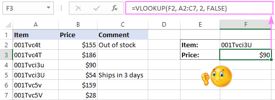
To perform a case-sensitive lookup in Excel, we combine the VLOOKUP, CHOOSE and EXACT functions:
This generic formula perfectly works in all situations. You can even look up from right to left, something that a regular VLOOKUP formula is unable to do. Kudos to Pouriya for suggesting this simple and elegant solution!
In our case, the real formulas go as follows.
To pull the price in F3:
=VLOOKUP(TRUE, CHOOSE({1,2}, EXACT(F2, A2:A7), B2:B7), 2, FALSE)
To fetch the comment F4:
=VLOOKUP(TRUE, CHOOSE({1,2}, EXACT(F2, A2:A7), C2:C7), 2, FALSE)
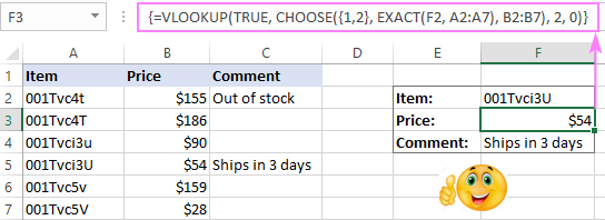
Note. In all Excel versions other than Excel 365, this only works as an array formula, so remember to press Ctrl + Shift + Enter to complete it correctly. In Excel 365, due to support for dynamic arrays, it also works as a regular formula.
How this formula works:
The core part that does the trick is the CHOOSE formula with nested EXACT:
CHOOSE({1,2}, EXACT(F2, A2:A7), C2:C7)
Here, the EXACT function compares the value in F2 against each value in A2:A7 and returns TRUE if they are exactly the same including the letter case, FALSE otherwise:
{FALSE;FALSE;FALSE;TRUE;FALSE;FALSE}
For the index_num argument of CHOOSE, we use the array constant {1,2}. As the result, the function combines the logical values from the above array and the values from C2:C7 into a two-dimensional array like this:
{FALSE,155;FALSE,186;FALSE,90;TRUE,54;FALSE,159;FALSE,28}
The VLOOKUP function takes it from there and searches for the lookup value (which is TRUE) in the 1st column of the 2-dimensional array (represented by the logical values) and returns a match from the 2nd column, which is the price we are looking for:
VLOOKUP(TRUE, {FALSE,155;FALSE,186;FALSE,90;TRUE,54;FALSE,159;FALSE,28}, 2, 0)
Case-sensitive XLOOKUP formula
Microsoft 365 subscribers can do a case-sensitive lookup in Excel with even a simpler formula. As you can guess, I'm talking about a more powerful successor of VLOOKUP - the XLOOKUP function.
Because XLOOKUP operates on lookup and return arrays separately, we do not need the two-dimensional array trick from the previous example. Simply, use EXACT for the lookup_array argument:
The last argument ("Not found") is optional. It just defines what value to return if no match is found. If you omit it, then a standard #N/A error will be returned in case the formula finds nothing.
For our sample table, these are the case-sensitive XLOOKUP formulas to use.
To get the price in F3:
=XLOOKUP(TRUE, EXACT(F2, A2:A7), B2:B7, "Not found")
To extract the comment F4:
=XLOOKUP(TRUE, EXACT(F2, A2:A7), C2:C7, "Not found")

How this formula works:
Like in the previous example, EXACT returns an array of TRUE and FALSE values, where TRUE represents case-sensitive matches. XLOOKUP searches the above array for the TRUE value and returns a match from the return_array. Please note, if there are two or more exactly the same values in the lookup column (including the letter case), the formula will return the first found match.
XLOOKUP limitation: available only in Excel 365 and Excel 2021.
SUMPRODUCT - case-sensitive lookup to return matching numbers
As you understand from the heading, SUMPRODUCT is yet another Excel function that can do a case-sensitive lookup, but it can return numeric values only. If this is not your case, then jump to the INDEX MATCH example that provides a solution for all data types.
As you probably know, Excel's SUMPRODUCT multiplies components in the specified arrays and returns the sum of the products. Since we want a case sensitive lookup, we use the EXACT function to get the first array:
=SUMPRODUCT((EXACT(A2:A7,F2) * (B2:B7)))
Regrettably, the SUMPRODUCT function cannot return text matches since text values cannot be multiplied. In this case, you will get a #VALUE! error like in cell F4 in the screenshot below:
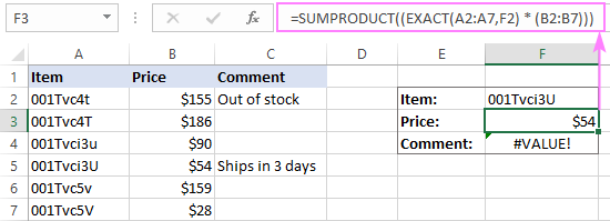
How this formula works:
Like in the VLOOKUP example, the EXACT function checks the value in F2 against all the values in A2:A7 and returns TRUE for case-sensitive matches, FALSE otherwise:
SUMPRODUCT(({FALSE;FALSE;FALSE;TRUE;FALSE;FALSE}*{155;186;90;54;159;28}))
In most formulas, Excel evaluates TRUE to 1 and FALSE to 0. So, when SUMPRODUCT multiplies the elements of the two arrays in the same positions, all non-matches (FALSE) become zeros:
SUMPRODUCT({0;0;0;54;0;0})
As the result, the formula returns a number from column B that corresponds to the exact case-sensitive match in column A.
SUMPRODUCT limitation: can return numeric values only.
INDEX MATCH - case-sensitive lookup for all data types
Finally, we are close to getting a limitation-free case-sensitive lookup formula that works in all Excel versions and on all data sets.
This example comes last not only because the best is saved for the last, but also because the knowledge you've gained in the previous examples may help you understand the case-sensitive MATCH INDEX formula better.
The combination of INDEX and MATCH functions is often used in Excel as a more flexible and versatile alternative to VLOOKUP. The following article does a good job (hopefully :) explaining how these two functions work together - Using INDEX MATCH instead of VLOOKUP.
Here, I will just remind you the key points:
- The MATCH function searches for the lookup value in the specified lookup array and returns its relative position.
- The relative position of the lookup value goes directly to the row_num argument of the INDEX function instructing it to return a value from that row.
For the formula to recognize text case, you just need to add one more function to the classic INDEX MATCH combination. Obviously, you need the EXACT function again:
The real formula in F3 is:
=INDEX(B2:B7, MATCH(TRUE, EXACT(A2:A7, F2), 0))
In F4, we are using this one:
=INDEX(C2:C7, MATCH(TRUE, EXACT(A2:A7, F2), 0))
Please remember that it only works as an array formula in all versions other than Excel 365, so be sure to enter it by press the Ctrl + Shift + Enter keys together. If done correctly, the formula will get enclosed in curly braces like shown in the screenshot below:
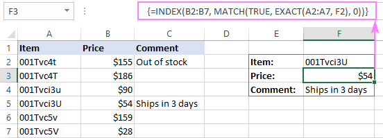
How this formula works:
Like in all previous examples, EXACT returns TRUE for each value in A2:A7 that exactly matches the value in F2. Since we use TRUE for the lookup_value of MATCH, it returns a relative position of the exact case-sensitive match, which is precisely what INDEX needs to return a match from B2:B7.
Advanced case-sensitive lookup formula
The above-mentioned INDEX MATCH formula looks perfect, right? But in fact, it is not. Let me show you why.
Suppose a cell in the return column corresponding to the lookup value is blank. What shall the formula return? Nothing. And now, let's see what it actually returns:
=INDEX(C2:C7, MATCH(TRUE, EXACT(A2:A7, F2), 0))
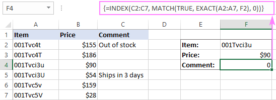
Oops, the formula returns a zero! Maybe, it's not really important when dealing solely with text values. However, if your worksheet contains numbers and some of them are real zeros, this is a problem.
In truth, all other lookup formulas discussed earlier behave in the same way. But now you want an impeccable formula, don't you?
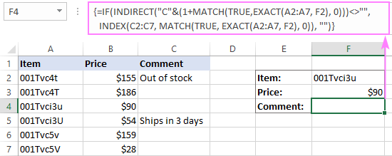
To make the case-sensitive INDEX MATCH formula absolutely perfect, you wrap it in the IF function that checks whether a return cell is blank and returns nothing in this case:
=IF(INDIRECT("C"&(1+MATCH(TRUE,EXACT(A2:A7, F2), 0)))<>"", INDEX(C2:C7, MATCH(TRUE, EXACT(A2:A7, F2), 0)), "")
In the above formula:
- "C" is the return column.
- "1" is the number that turns a relative position of the cell returned by the MATCH function into a real cell address.
For example, the lookup array in our MATCH function is A2:A7, meaning the relative position of cell A2 is "1", because this is the first cell in the array. But in reality, the lookup array begins in row 2. To compensate the difference, we add 1, so the INDIRECT function will return a value from the right cell.
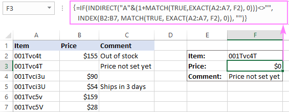
The below screenshots demonstrate the improved case-sensitive INDEX MATCH formula in action.
If the return cell in empty, the formula outputs nothing (an empty string):
If the return cell contains a zero, the formula returns 0:
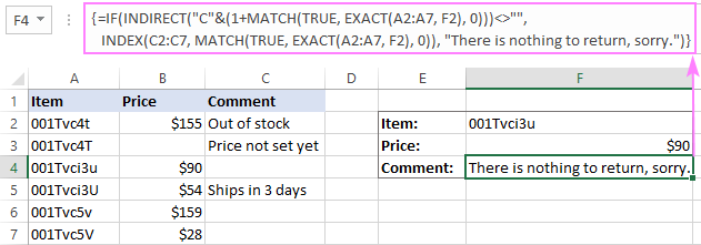
If you'd rather display some message when a return cell is blank, replace an empty string ("") in the last argument of IF with some text:
=IF(INDIRECT("C"&(1+MATCH(TRUE, EXACT(A2:A7, F2), 0)))<>"", INDEX(C2:C7, MATCH(TRUE, EXACT(A2:A7, F2), 0)), "There is nothing to return, sorry.")
Do case-sensitive VLOOKUP an easy way
The users of our Ultimate Suite for Excel have a special tool that makes looking up in large and complex tables easier and stress-free. The best thing is that Merge Two Tables has a case-sensitive option, and the below example shows it in action.
Suppose you want to pull Qty. from the Lookup table to the Main table based on unique Item ID's:

What you do is to run the Merge Tables wizard and perform these steps:
- Select the main table into which to pull new data.
- Select the lookup table where to look for the new data.
- Choose one or more key columns (Item ID in our case). And be sure to check the Case-sensitive matching box.

- The wizard will walk you through the remaining three steps where you specify which columns to update, which columns to add and choose some additional options if needed.
A moment later, you will get the desired result :)

That's how to lookup in Excel taking into account the text case. I thank you for reading and hope to see you on our blog next week!
Practice workbook for download
Case-sensitive VLOOKUP examples (.xlsx file)
 by
by
42 comments
Thank you Svetlana,
Very interesting use case and clear explanations of the different options.
However I would suggest an alternative to the usage of 'indirect' in the 5th option to avoid the conversion of "" (empty cell) into a "0" result using just an 'IF' function, meaning :
= IF(INDEX(INDEX(C2:C7, MATCH(TRUE, EXACT(A2:A7, F2), 0))="","",INDEX(C2:C7, MATCH(TRUE, EXACT(A2:A7, F2), 0)))
So we get "" if there no comment and "0" in case of "0" without the disavantage of INDIRECT (which is not flexible when inserting columns od moving ranges).
It seems it work well on my side at least.
'=INDEX('Raw Data'!$AH$5:$AH$99,MATCH(A3,'Raw Data'!$A$5:$A$99,0))
I have this formula above where when I insert a new column in " Raw Data" Sheet, Column AH moves to AI, I wanted to keep AH column constant even when a new column is inserted. Thanks!
Hi! If I understand your task correctly, the following tutorial should help: Using Excel INDIRECT function to lock a cell reference. I hope it’ll be helpful. If something is still unclear, please feel free to ask.
I think that we can use vlookup through this way:
=VLOOKUP(MAX(EXACT(D5,$N$5:$N$10)*ROW($N$5:$N$10)),$O$5:$P$10,2)
Discovered my problems - in your seminar the section explaining the "Return Column" the equation starts with "=IF(INDIRECT("C" than the Explanation is "In the above formula: "B" is the return column" Was confused at first. As I review / read your seminar, I reproduce all analyzes - as of now got all formulas to work. Thank you.
Hi Waldo,
Of course, it's "C" not "B". Thank you for pointing that out, fixed! And sorry for the confusion.
Spent a few hours attempting to get this formula to work and no luck. Even tried your "Practice Workbook Download". Is there a Excel version requirement? Maintain 2010 version
Formula
{=IF(INDIRECT("A"&(1+MATCH(TRUE,EXACT(A2:A7,F2),0)))"",INDEX(B2:B7,MATCH(TRUE,EXACT(A2:A7,F2),0)),"")}
and
=IF(INDIRECT("C"&(1+MATCH(TRUE, EXACT(H279:H284, N278), 0)))"", INDEX(J279:J284, MATCH(TRUE, EXACT(H279:H284, N278), 0)), "There is nothing to return, sorry.")
Also, if you change the "Item" selection to an "Item" with a "Comment" the "There is nothing to return, sorry" stays.
Thoughts
Thanks
If the "Item" listing starts on Cell H35, does the - Indirect("A" change to - Indirect("H" or does "A" stay?
Hi!
I can't check your formula, but Indirect("С" should be replaced with Indirect("H"
The letter must match the column you are searching.
Hello Svetlana: Thank you for an informative tutorial.
My issue resolves around using the "REMOVE DUPLICATES" function in Excel. I have a list of Salesforce ID's . Let's say a thousand with lower and upper cases in the ID. When I use the "Remove Duplicates" function it, of course, removes unique ID's (when the ID contains lower and upper case for the same letter).
How would you resolve this issue?
Thank you in advance for your assistance.
Tony
Hello!
In step 3 in the Duplicate Remover, enable the "Case-sensitive match" option. Then the tool will distinguish the case of characters.
A standard Excel function cannot do this.
The lookup example will not match the 1st item in row 2. It returns the last record. I switched to the Lookup(1,1/Exact formula and that seemed to work all around. Even in you test excel file it does the same.
Thanks - very informative!
Hi Tim,
Thank you very much for your feedback! The LOOKUP formula is wrong indeed, my apologies. The point is that for correct work, the LOOKUP function requires sorting the lookup array (lookup_vector) from A to Z. But in my formula, the lookup array was returned by the EXACT function, and obviously it wasn't sorted. I just don't know where my eyes were back in 2014 when I wrote that formula :(
Anyway, the erroneous example is removed, and we'll update the sample workbook ASAP.
Your contents is perfect and very useful.
I think that we can use vlookup through this way:
{=VLOOKUP(TRUE,CHOOSE({1,2},EXACT($E$3,A2:A8),B2:B8),2,0)}
Hi Pouriya,
What an elegant and effective solution! Thank you so much for sharing!
This is so useful and opens up new ways to think about and approach problems. Quite beautiful. Thank you.
Thanks Svetlana - this is great.
Can I ask please (this seems to have been asked before) - I need to do the same for Salesforce ID's, which use case to make them unique.
They are 15 characters long (always) - is it simply the case of adding "code" to your formula?
i.e =CODE(MID(D2,1,1)) & CODE(MID(D2,2,1)) & CODE(MID(D2,3,1)) & CODE(MID(D2,4,1)) & CODE(MID(D2,5,1)) & CODE(MID(D2,6,1)) & CODE(MID(D2,7,1)) & CODE(MID(D2,8,1)) & CODE(MID(D2,9,1)) & CODE(MID(D2,10,1)) & CODE(MID(D2,11,1)) & CODE(MID(D2,12,1)) & CODE(MID(D2,13,1)) & CODE(MID(D2,14,1)) & CODE(MID(D2,15,1)) & IFERROR(CODE(MID(D2,16,1)),"")
I've tried this - Excel really doesn't like it. I have 145,000 rows, and it seems to consider every single one of the new "unique" codes to be duplicates!
Thanks, Svetlana!!
I am very thankful to you for your nice efforts. carry on..
There is an unfortunate misspelling in the 2nd paragraph. I think you are trying to say "meaning it treats lowercase and UPPERCASE characters as identical." But the word "treats" is missing an "r".
Thanks for this very informative post.
Hi Brady,
Thank you for pointing that out! Fixed.
I found a simple way to use VLOOKUP() + EXACT() functions for Case Sensitive validation:
Lets say in Worksheet A I have a list of Topics in Column A
Lets say in Worksheet B I have a list of students (Col A) and in column B the Topic they choose. I want to make sure they used an existing Topic with Case Sensitivity
Step 1: in Worksheet B I add a Dummy Column C with formula =VLOOKUP(B2,topics!$A:$A,1,FALSE) . this will get me the name of the Topic in Topic Worksheet but not case sensitive
Step2: in Worksheet B I add another Dummy Column D with formula =EXACT(B2,C2) this will compare the name I used as Topic to the name I found via Vlookup. If value if FALSE it means that there is issue with case sensitive letters (you can add conditional format to color it)
The first solution of helper column is really helpful particularly when all the look-up values have same number of character, as in my case.
! (among many others) have identical returns for =code(mid(B1,1,1))&code(mid(B1,2,1))
Svetlana, you are wonderful. I too was looking for a solution to using vLookup on Salesforce IDs. While there is a 15 char to 18 char conversion site that can make vLookup work, it takes extra effort. Your ...match(true,exact)... formula works much faster and simpler. Thanks!
I just want to say that this article saved my life during a Salesforce migration, where many unique IDs require case sensitivity. This workaround made everything possible.
Many thanks Svetlana, worked for me, this is a common problem faced by many and I am sure this post will be of great help.
I want to how is interest calculated by banks in savings and current a/C with regular deposits and withdrawals on monthly basis?
Guys a very easy formula there to do this using code formula. Using code formula you can convert those case sensitive item into unique numbers.