It will take you about 10 minutes to read this article and in the next 5 minutes (or even faster if you choose the 2nd solution described in the article) you will easily compare two Excel columns for duplicates and remove or highlight the found dupes. Okay, the countdown is started!
Excel is a very powerful and really cool application for creating and processing large arrays of data. Now that you have lots of workbooks with a pool of data, or maybe just one huge table, you may want to compare 2 columns for duplicates and then do something with found entries, for example delete duplicate rows, color dupes or clear the contents of duplicated cells. These two columns may be located in one table, contiguously or non-contiguously, or they may reside in 2 different worksheets or even workbooks.
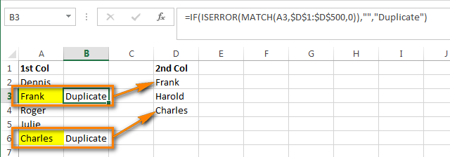
Say, you have 2 columns with people names - 5 names in column A and 3 names in column B, and you want to compare data between these two columns to find duplicates. As you understand, this is bogus data just for a quick example; in real worksheets you usually have thousands and tens of thousands of entries.
Variant A: Both columns are located on one sheet, in a single table: Column A and Column B
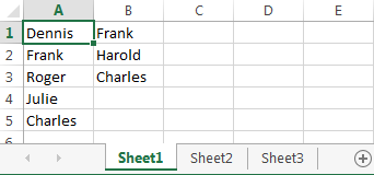
Variant B: Two columns are located on different sheets: Column A in Sheet2 and Column A in Sheet3

The built-in Remove Duplicate tool available in Excel 2016, Excel 2013 and 2010 cannot handle this scenario because it cannot compare data between 2 columns. Furthermore, it can only remove dupes, no other choice such as highlighting or coloring is available, alas :-(.
Further on, I am going to describe 2 possible ways of comparing two Excel columns that let you find and remove duplicate entries:
Compare 2 columns to find duplicates using Excel formulas
Variant A: both columns are on the same list
- In the first empty cell, in our example this is Cell C1, write the following formula:
=IF(ISERROR(MATCH(A1,$B$1:$B$10000,0)),"Unique","Duplicate")
In our formula, A1 is the first cell of the first column that we want to use for comparison. $B$1 and $B$10000 are the addresses of the first and the last cell of the 2nd column that you want to compare against.Pay attention to the absolute cell reference - dollar signs ($) preceding the column letters and row numbers. I use the absolute reference on purpose, in order for the cell addresses to remain unchanged when copying the formula.
If you want to find dupes in Column B, swap the column names so that the formula looks like this:
=IF(ISERROR(MATCH(B1,$A$1:$A$10000,0)),"Unique","Duplicate")Instead of "Unique"/"Duplicate" you can write your own labels, e.g. "Not found"/"Found", or leave only "Duplicate" and type "" instead of "Unique". In the latter case, you will have empty cells next to cells for which duplicates were not found, I believe such presentation is more convenient for data analysis.
- Now let's copy the formula to all cells of column C, up to the last row that contains data in column A. To do this, put the cursor to the lower right corner of cell C1, and the cursor will change to a black cross, as shown in the image below:

Click the left mouse button and holding it down drag the border downward selecting all cells where you want to copy the formula. When all needed cells are selected, release the left mouse button:

Tip: In large tables, it is faster to copy the formula using shortcuts. Click on cell C1 to select it and press Ctrl + C (to copy the formula to clipboard), then press Ctrl + Shift + End (to select all non-empty cells in Column C), and finally hit Ctrl + V (to paste the formula into all selected cells).
- Awesome, all duplicated cells are flagged as "Duplicate":

Variant B: two columns are on different worksheets (workbooks)
- In the 1st cell of the 1st empty column in Sheet2 (column B in our case), write the formula:
=IF(ISERROR(MATCH(A1,Sheet3!$A$1:$A$10000,0)),"","Duplicate")Where Sheet3 is the name of the sheet on which the 2nd column is located, and $A$1:$A$10000 are the addresses of the first and last cells of that 2nd column.
- Similar to Variant A.
- We have the following result:

Click to download the worksheet with the above examples and the formula to compare 2 columns to find duplicates.
Working with found duplicates
Perfect, we have found the entries in the first column (Column A) that also exist in the second column (Column B). Now we need to do something with them :)
It would be rather ineffective and would take too much time to look through the entire table and review the duplicate entries manually. There are much better ways.
Show only duplicated rows in Column A
If your columns do not have headers, you need to add them. To do this, put the cursor on the number indicating the 1st row and it will change to a black arrow as shown in the screenshot:

Right click the selected row and choose "Insert" from the context menu:

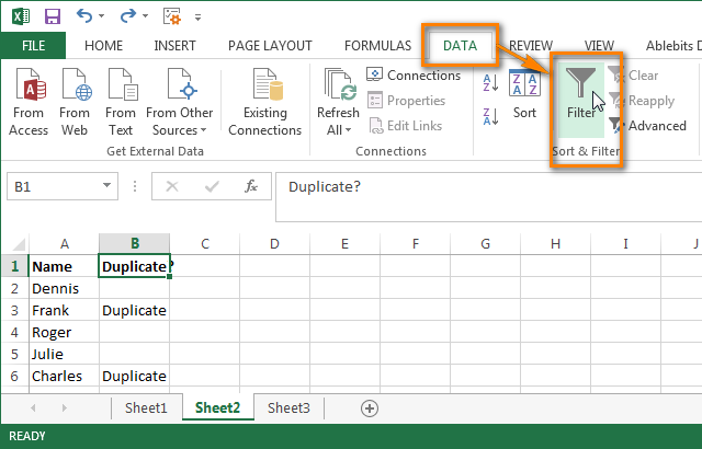
Give names to your columns, e.g. "Name" and "Duplicate?". Then switch to the Data tab and click Filter:
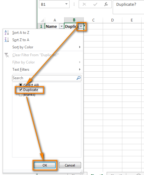
After that click a tiny grey arrow next to "Duplicate?" to open a drop down list, uncheck all items other than Duplicate in that list, and click OK:
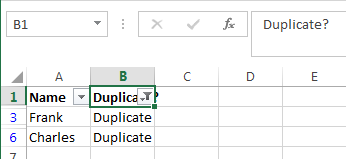
That's it, now you see only those cells of Column A that have duplicated values in Colum B. There are only three such cells in our test worksheet, as you understand in real sheets there are likely to be more, far more of them:
In order to display all rows of Column A again, click the filter symbol in Column B that now looks like a funnel with a tiny arrow ![]() and check "Select all". Alternatively, you can do the same via Data tab -> Select & Filter -> Clear, as shown in the screenshot:
and check "Select all". Alternatively, you can do the same via Data tab -> Select & Filter -> Clear, as shown in the screenshot:

Color or highlight found duplicates
If the "Duplicate" flag does not suffice for your purposes and you want to mark duplicated cells by font color or fill color or in some other way…
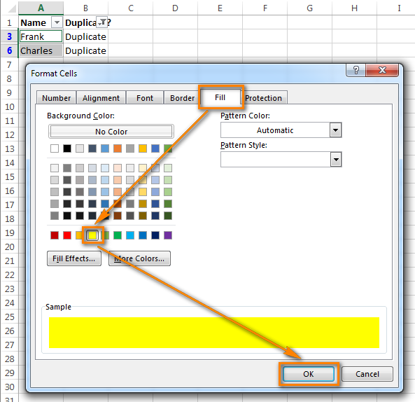
Then filter the duplicates as explained above, select all filtered cells and press Ctrl + F1 to open the Format Cells dialog box. As an example, let's change the background color of duplicated rows to bright yellow. Of course, you can change the background color of cells using the Fill color option on the Home tab, but the advantage of the Format Cells dialog box is that it lets you make all formatting changes at a time:
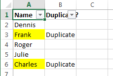
Now you definitely won't miss a single duplicated cell:
Remove duplicates from the first column
Filter your table so that only cells with duplicated values show up, and select all those cells.
If 2 columns you are comparing are located on different worksheets, i.e. in separate tables, right-click the selected range and choose "Delete Row" from the context menu:
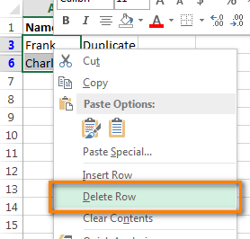
Click OK when Excel will ask you to confirm that you really want to "Delete entire sheet row" and then clear the filter. As you can see, only the rows with unique values are left:
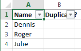
If 2 columns are located on one worksheet, next to each other (adjacent) or not touching each other (nonadjacent), the removing duplicates is a bit more complex. We cannot delete entire rows that contain duplicate values because this would delete corresponding cells in the 2nd column too. So, in order to leave only unique entries in Column A, you do the following:
- Filter the table so that only duplicated cells are displayed and select all those cells. Right click the selection and choose "Clear contents":

- Clear the filter.
- Select all cells in Column A starting from cell A1 up to the last cell that contains data.
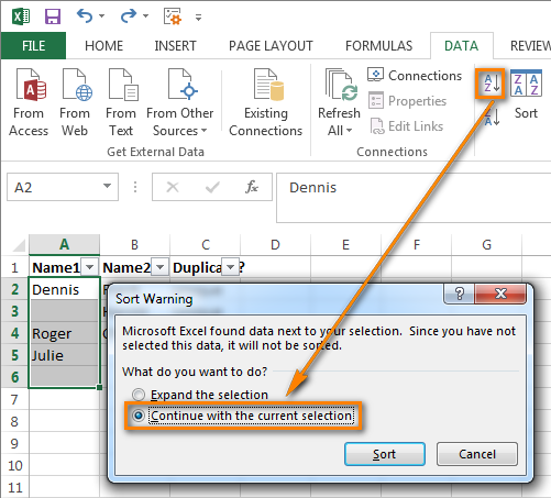
- Go to the Data tab and click Sort A to Z. In the dialog window that opens, choose "Continue with the current selection" and click Sort:
- Delete the column containing the formula because you do not need it any longer, only "Uniques" are left there by now.
- That's all, now Column A contains only unique data that do not exist in Column B:

As you see, it's not so difficult to remove duplicates between two Excel columns using formulas. Though it's very time-consuming and boring process to write and copy the formula, apply and clear the filter every time you need to compare 2 columns in your worksheets. The other solution I am going to bring to your attention is much simpler and will take just a fraction of time we've spent on the first method. I believe you will find more pleasant things to spend the saved time on ;)
Compare 2 Excel columns for duplicates using a visual wizard
And now let me show you how to compare two columns for duplicates by using our Dedupe tools for Excel.
- Open the worksheet (or worksheets) where the columns you want to compare are located.
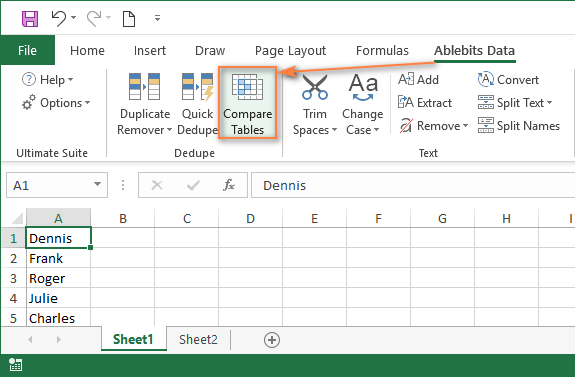
- Select any cell within the 1st column, switch to the Ablebits Data tab and click the Compare Tables button:
- On step 1 of the wizard, you will see that your first column is already selected, so simply click Next.
Note. If you want to compare not just 2 columns, but 2 tables, you need to select the entire first table in this step.
- On step 2 of the wizard, select the 2nd column that you want to compare against. We choose Sheet2 in the same workbook. In most cases, the smart wizard selects the 2nd column automatically, if for some reason this does not happen, select the target column using the mouse. If you are comparing entire tables, select the whole 2nd table.

- Choose to find Duplicate values:

- Pick the pair of columns you want to compare:

Tip. If you are comparing tables, you can choose several column pairs for comparison, for example, first and last name. For more details, please see How to remove duplicates from two Excel spreadsheets.
- And finally, you are to decide what you want to do with found dupes. You can choose to delete the duplicate entries, move or copy them to another worksheet, add a status column (the result will be similar to our first solution with Excel formulas), highlight duplicates, or just select all cells with duplicated values:
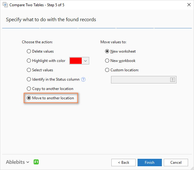
Tip. Do not choose to delete duplicates, especially if you are using the tool for the first time. Instead, choose to move dupes to another worksheet. This will remove duplicates from the first table, but gives you a chance to review the list of entries recognized as duplicates. When comparing by several matching columns in large tables, it may happen that you accidentally forgot to select a key column with unique data, and moving duplicates will prevent an irretrievable loss of data.
- Click Finish and enjoy the result. What we have now is a nice, clean table with no duplicates:

Remember the previous solution and feel the difference :) It is fast and easy indeed to dedupe your worksheets with Compare Two Tables. In fact, it will take you less time than you've spent on reading this article.
Currently, Compare Tables is part of our Ultimate Suite for Excel, a collection of 70+ professional tools that covert over 300 use cases. The clock is ticking, so hurry up and download it right now!
If you have questions or something is left unclear, please drop me a comment and I'll happily elaborate further. Thank you for reading!
 by
by
2 comments
Thank you so much Alexander. You saved a big project where we were racking our heads on removing duplicates from a huge volume data. Is your first method useful in selecting multiple columns? If you happen to see my message, please reply.
And also, the tool provided by Ablebits, is it open source or paid? Please let me know. Thank you.
Hello Julie,
Yes, the first method can be used to compare 2 lists / tables by multiple columns, but it will require extra effort.
First, you need to create a helper column in each list. In the helper column, combine the data from the columns you want to compare by.
Assuming your first table includes columns A, B, C and your second table - columns K, L, M; row 1 is column headers, and data starts in row 2. You want to compare columns A + B with columns K + L.
In cell D2, enter the formula = A2&B2 and copy it down to the end of the table.
In cell N2, enter the formula = K2&L2 and copy it through the entire table.
For more information, please see this comprehensive tutorial on concatenating cells.
Then, in cell E2, enter the formula discussed in the first method:
=IF(ISERROR(MATCH(D2,$N$2:$N$10000,0)),"","Duplicate")
Compare Tables is part of Ultimate Suite for Excel, which is a paid product. It includes over 60 tools to handle more than 300 different tasks. And it has taken quite us a lot of time and resources to develop it :)
You can read more about Ultimate Suite here:
https://www.ablebits.com/excel-suite/index.php
On the above page, you can also download a 14-day fully functional trial version to decide whether it is worth buying a license.