In this quick tip you will learn about 2 fast ways to enter the same formula or text into several Excel cells at a time. It is very useful if you need to insert the formula to all cells in a column or fill all blank cells in a table with the same value (e.g. "N/A"). Both tricks work in Microsoft Excel 365 - 2007.
Knowing these simple techniques will save you a lot of time that you can spend on more enjoyable things.
Select all the cells where you want to enter the same data
Here are the quickest ways you can select cells:
Select the entire column
- If your data are in a full-fledged Excel table, just click on any cell in the column and press Ctrl+Space.
- If you have a simple range (when you click on any cell with the data, you don't see "Table Tools" tab in the top-right corner of the Excel ribbon):

Note.
Note: Unfortunately, simply pressing Ctrl+Space will select all the cells in the column, i.e. from C1 to C1048576, even if only cells C1-C100 contain data.Put the cursor to the first cell in the column (or the second one if your Table has headers), then press Shift+Ctrl+End to go to the end of your table, hold Shift and press the Left key repeatedly until only the needed column gets selected.
This is the fastest way to select all the cells in the column, especially if the column contains several blank cells between the data.
Select the entire row
- If your data are in a full-fledged Excel table, just click on any cell in the row and press Shift+Space.
- If you have a simple range, click on the last cell in the row, then press Ctrl + Home.
Select several cells
Hold Ctrl and left-click on all cells that you want to fill with data.
Select the whole table
Click on any cell in your table and then press Ctrl+A.
Select all cells in a worksheet
Press Ctrl+A, then Ctrl+A again.
Select blank cells within a certain area (row, column, table)
Select the area you need (see below), e.g. the whole column.
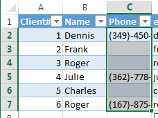
Press F5 to bring up the "Go To" dialog and click on the Special… button in that dialog.
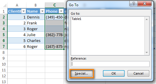
Select the "Blanks" radio button in the "Go To special" window and click OK.
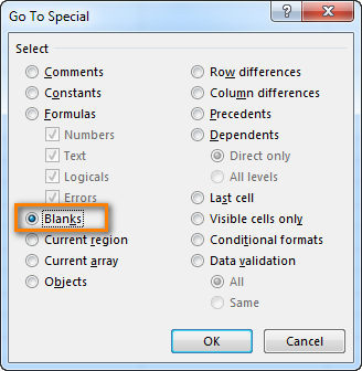
You will get back to Excel and see that only blank cells in the selected area are highlighted. That's right; it is faster to select 3 blank cells by clicking on them with your mouse cursor. But what if you have more than 300 blanks randomly distributed between 10000 cells :)?
The fastest way to insert a formula into the entire column
You have a large table and you want to add a new column with some formula. For example, you get a list of links (new backlinks to www.ablebits.com :) ) and you want to extract the domain names from these links for further work.

- Convert your range to an Excel table. Select any cell within your data range and press Ctrl+T to bring the "Create Table" dialog (the shortcut is Ctrl+L in Excel 2003). If your data have column titles, make sure the checkbox "My table has headers" is selected. Usually Excel recognizes your table headers automatically, if not, check this checkbox manually.

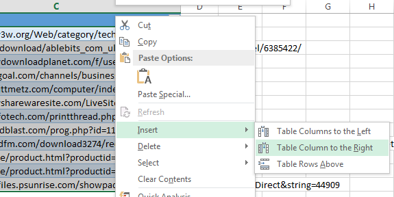
- Insert a new column into your table. It is a lot easier to add a new column to a table than to a simple data range. Just click on any cell in the column next to where you want to add a new one and choose Insert > Table Column to the Right ( or "Table Column to the Left").
- Name the newly added column.
- Enter your formula in the first cell of the new column. I'll use the following formula for extracting domain names in my example:
=MID(c2,FIND(":",c2,"4")+3,FIND("/",c2,9)-FIND(":",c2,"4")-3)
- Press Enter. Voila! Excel automatically fills all blank cells down your column with the same formula
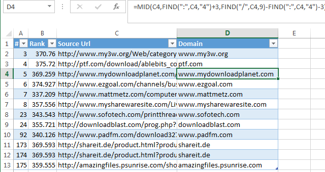
If you want to switch back from a table to a simple range for some reason (I don't know any :) ), select any cell in your table, then press the "Convert to range" button on the Design tab.

You can apply this tip only if all cells in the column are blank, so the best way is to add new columns. The next tip is universal.
Insert the same data into multiple cells using Ctrl+Enter
Select the cells that you want to fill with the same data in your Excel worksheet. Please see the tips above for quick data selection.
Say, we have a table with a list of our customers (this is a fake list, of course :) ). There is a column listing the websites from which our customers come. We want to fill the blank cells with "_unknown_" to make filtering easier in the future:

- Select all the blank cells in a column.

- Press F2 to edit the last selected cell and type some data: it can be text, a number, or a formula (e.g. "_unknown_")

- Press Ctrl+Enter instead of Enter. All the selected cells will be filled with the data that you typed.

If you know more tricks that speed up data input, please share them in the comments. I'll be happy to add them with your authorship to this article.
 by
by
167 comments
THE FASTEST WAY TO INSERT A FORMULA INTO (THE ENTIRE or part of) A COLUMN, or even in scattered cells
is not the one suggested above (defining a table etc. etc.), I believe, but the following:
1) Mark the column (or the range - or even the scattered cells [usually in the same column] - where you want the formula/function to be inserted)
2) Having the cells (i.e. full or part of the column) marked, type in the formula bar (or even directly in the active cell) the function/formula you want.
3) Press CTRL-ENTER.
4) BOOM !!!
It is exactly the same method one uses to insert the same text/number/date/etc. now even formulas and functions into multiple cells.
Of course the suggested way above with defining the table is more "structured", I could say, but more restrictive (what if I want to enter the formula in most cells of the column but not ALL of them?) and certainly not the fastest.
Am I not correct or I missed something?
Hello,
I have a tracker that is used to track new client policies and premium amounts, for the current month. We need the info roll over to each month without having to copy and paste manually every time a new policy is written. But if client cancels policy on a set date, we need the rollover to stop. For example: on January, i write 5 new policies, i want those 5 to copy over to every month, a long with the premiums they pay monthly, but lets say they cancel in April, i want it to no longer copy over past april. Can you please help? not sure if this can be done or if i would need a macro instead. any assistance is greatly appreciated. thank you in for your time.
Hi! To automatically copied values from one worksheet to another worksheet, you can use a macro. But that is beyond the scope of the help we provide in this blog. You can also try to extract data by condition from another worksheet using the FILTER function. Without seeing your data, it is impossible to give you an example of such a formula.
i need to copy the same date from sheet 1 to sheet 4.for example if sheet 1 has a name typed i hope for this name to be typed into sheets 2-4 automatically, not manually..is there such a formula
Hi! If I understand your task correctly, this guide may be helpful: Excel reference to another sheet.
Hi, I have a model already built but I need to add another row with a formula already in it into roughly 120 different places in the model. Is there a quick way to do this?
Thanks!
Hi! This article describes a quick way to insert values into cells or formulas: Using Excel Find and Replace in the most efficient way. It might be helpful.
I have 2500 rows in my table, in a certain column i need to add "-00" at the end of my value. Please advise how can i do that using a formula in 2500 rows of column.
Hi! To add text to a cell value, use the concatenation operator & or the CONCAT function.
For example, A1&"-00".
You can add text to each of the 2500 cells with a couple of clicks without formulas using the Add Text tool. It is available as a part of our Ultimate Suite for Excel that you can install in a trial mode and check how it works for free.
Hi
Colom (A) Colom(B)
(NAME) (REGION)
A USA
B ASIA
When i type name C under name coloum how can i select region as USA in region coloum without typing
thanks
Hi! You can write a nested IF formula with multiple conditions in column B to automatically insert a value depending on the value in column A. If there are a very many conditions, I recommend using IFS function instead of multiple IF.
I want to paste a 21 digits numbers like '********************' in excel. I want paste the exact numbers as per columns? Can you helped me solved it? What if I used the 'if' FUNCTIONS. Will it work? Surely vLOOKUP doesn't help as it have multiple columns and rows. How to paste the correct numbers in the same rows along with the contained multiple rows. Thanking you in advance.
R-1 S/No R2 ID No (containing 20+ digit) R3 Order ID (same containing 20+ digit not in ascending or descending) R4 Name R5 Address and so on
C1 1-2000+ C2 12345678910111213142 C3 12345678910111213142 C4 John C5 Oakland, etc...
select the particular cell and drag the data so it will be
Hi! To insert a text string into text, you can try using the REPLACE and SUBSTITUTE functions. They can replace part of the text with the required text string or insert a text string at the target position. I hope it’ll be helpful.
If this does not help, explain the problem in detail.
It contains 2500 rows, 20 or more columns. I'm asking vice-versa on columns and rows also. Please help me....
HELLO
I have panel data set if 100 categories of imported products which are in a way that
product 1 volume RCA (A) RCA (B) product 2 volume RCA (A) RCA (B).... upto 100 products
year 2011
2012
2013
upto
2020
i want this data to be in vertical form like
product 1 volume RCA( A) RCA (B)
year 2011
year 2012
year2013
upto 2020
product 2
year 2011
year 2012
year 2013
upto 2020
please help urgently
additional information of above query
each product has 3 columns and 11 rows. i do not want to take their transpose as order of columns is correct. order of years is also set. only set of data of products should stack on each other. like book 1 should be on the book 2 in the shelf not their pages.
Good morning, I would like to clone two rows. If changes are made to row 2 can that reflect in row 48?
Hi,
Suppose you have 5 cells in Excel & each cell has a date. Now I want to make a formula in another cell (cell no. 6) that is-
if cell 1 has a date, then the formula cell will show "Received" & all others will have blank. Again, if cell 2 has a date, then the formula cell will show "Sent" and all other cells will remain blank. But not cell 1 and cell 2. I mean blank will be 3,4,5.
Can you please help me?
Hi! An Excel formula can only change the value of the cell in which it is written. Use the IF function.
=IF(A1<>"","Received","")
Good afternoon,
I have a question pertaining to separating first and last names and combining them. You see, I know how to separate and combine them, however the data I have has names either first then last, or last then first, all in one row. What makes this difficult is that I do not know if, and how, Excel can auto sort the names without me having to fix the backward names manually. Would there happen to be a known solution to this dilemma?
Hi! Excel cannot automatically recognize the first name from the last name.
Hi I have one question on how to make the same value in 5 rows. And there are 62 different values and that means there would be 310 rows for it.
Hi! To create a series of numbers, each of which is repeated 5 times, use the SEQUENCE function. For example,
=CEILING(SEQUENCE(310,1,1,1)/5,1)
If you have a list of values, try using these instructions: How to get random sample in Excel without duplicates:
=INDEX(SORTBY(A2:A10, RANDARRAY(ROWS(A2:A10))), CEILING(SEQUENCE(310,1,1,1)/5,1))
Hi, I need help finding a formula. Have tried different ones it sends me an error (SPILL).
Sheet One I have four columns, all integer values. Column A has Plots, Column B has Temp1, Column C has Temp2 and Column D has Temp3. There are 1500 for each plot, total 45k, and I need to put their corresponding values of each Temp which are coming from another sheet (Test-Temp Sheet, each temp on different column). Any idea? Thanks!
Sheet One looks like this....
Plot Temp1 Temp2 Temp3
1
1
1
1
Test-Temp Sheet looks like this...
Plot Temp1 Temp2 Temp3
1 1.56 2.08 0.52
2 4.68 2.6 0.1
3 6.3 8.52 -0.52
Thanks!
Hi! Please clarify your specific problem or provide additional details to highlight exactly what you need. As it's currently written, it's hard to tell exactly what you're asking.
Thankyou for explaining the method ....filling same number in multiple cells is what i was looking for and got it in your website ..great going
Hi, i was wondering if you can help. I have a list of website links, lets say they all begin with this "www.onlinegames.com/play/" and after "play" its the name of the game (the full link might look like this : www. onlinegames.com/play/random-game-1 , www. onlinegames.com/play/new-random-game-1, www. onlinegames.com/play/random-game-2 etc.)
I don't initialy have them on the spreadsheet and need to introduce them BUT, I do have the column with the game name (random-game-1, new-random-game-1,random-game-2 etc. ) So the spreadsheet is like this Col A = Full Marketing Name, Col B = random-game-name, Col C = Website links
If I copy the text "www. onlinegames.com/play/" in a random cell outside these columns, how can I use that in a formula that automatically copies "www.onlinegames.com/play/" + then adds "random-game-name" from Col B?
Hello!
Here is the article that may be helpful to you: How to select random sample in Excel.
Is there any way to add "text", for multiple cells, like I want to add colons and comma before and after the text,
Hi,
Is there anyway that i can get one cell (B17) to paste into another cell (G17) when clicking a cell (A1)?
Thank you
Hi!
Excel functions only work on the current cell. Your task can be solved with a VBA macro.
Looking to be able to put same data in two cells using either cell as the data entry cell.
example
A5 is a numbered cell that will change on occasion. In another part of the sheet cell Q5 represents the same data as cell A5. I want to be able to change that data in either cell.
Today A5 and Q5 would be the number 10, but tomorrow I need them to be changed to 12 but I don't want to have to go to each cell to make the change because the two cells will always be equal to each other. I'd also like to be able to make the change in either location and have the other cell change automatically too.
in Q5, type = and click on A5. Whatever you type into A5 will be duplicated into Q5.
O, the kind soul!
I have been looking for that simple advice for hours and here it is!!!
Thank you very much!!!
Hi!
Have you tried the ways described in this blog post? If they don’t work for you, then please describe your task in more detail, I’ll try to suggest a solution.
Hi, can anyone tell me what command I can use to copy data of one cell to an entire single row. Basically, I want to achieve the below steps with command.
.....................................
Move or copy cells
Select the cells or range of cells that you want to move or copy.
Point to the border of the cell or range that you selected.
When the pointer becomes a Hand pointer , do one of the following:
To
Do this
Move cells
Drag the cells to another location.
Copy cells
Hold down OPTION and drag the cells to another location.
Hi everyone,
I have a spreadsheet with date columns. How do I input the same date in the column (i.e. C2:C20) without the date automatically increasing numerically every cell
Thanks
I have a row of data with different number values and I just to simply add 5 in each cell. Example I have 96 in A1 and 10 in A2 and want to add 5 so they will become 101 and 15. How can I do that without typing or calculating manually? Please help!
Hello!
How to paste and add/subtract/multiply/divide at a time - use Paste special.
I hope it’ll be helpful.