The tutorial explains all main features of Excel conditional formatting with examples. You will learn how to do conditional formatting in any version of Excel, efficiently use preset rules or create new ones, edit, copy and clear formatting.
Excel conditional formatting is a really powerful feature when it comes to applying different formats to data that meets certain conditions. It can help you highlight the most important information in your spreadsheets and spot variances of cell values with a quick glance.
Many users, especially beginners, find it intricate and obscure. If you feel intimidated and uncomfortable with this feature, please don't! In fact, conditional formatting in Excel is very straightforward and easy to use, and you will make sure of this in just 5 minutes when you have finished reading this tutorial :)
What is conditional formatting in Excel?
Excel Conditional Formatting is used to apply certain formatting to data that meets one or more conditions. Just like usual cell formatting, it lets you highlight and differentiate your data in various ways by changing cells' fill color, font color, border styles, etc. The difference is that it is more flexible and dynamic - when the data changes, conditional formats get updated automatically to reflect the changes.
Conditional formatting can be applied to individual cells or entire rows based on the value of the formatted cell itself or another cell. To conditionally format your data, you can utilize preset rules such as Color Scales, Data Bars and Icon Sets or create custom rules where you define when and how the selected cells should be highlighted.

Where is conditional formatting in Excel?
In all versions of Excel 2010 through Excel 365, conditional formatting resides in the same place: Home tab > Styles group > Conditional formatting.
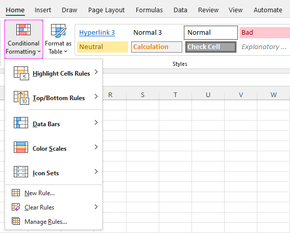
Now that you know where to find conditional formatting in Excel, let's move on and see how you can leverage it in your daily work to make more sense of the project you are currently working on.
For our examples, we will use Excel 365, which seems to be the most popular version these days. However, the options are essentially the same in all Excels, so you won't have any problems with following no matter what version is installed on your computer.
How to use conditional formatting in Excel
To truly leverage the capabilities of conditional format, you need to learn how to utilize various rule types. The good news is that whatever rule you are going to apply, it defines the two key things:
- What cells are covered by the rule.
- What condition should be met.
So, here's how you use Excel conditional formatting:
- In your spreadsheet, select the cells you want to format.
- On the Home tab, in the Styles group, click Conditional Formatting.
- From a set of inbuilt rules, choose the one that suits your purpose.
As an example, we are going to highlight values less than 0, so we click Highlight Cells Rules > Less Than…
- In the dialog window that appears, enter the value in the box on the left and choose the desired format from the drop-down list on the right (default is Light Red Fill with Dark Red Text).
When done, Excel will show you a preview of formatted data. If you are happy with the preview, click OK.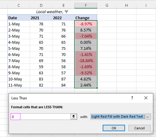
In a similar manner, you can use any other rule type that is more appropriate for your data, such as:
- Greater than or equal to
- Between two values
- Text that contains specific words or characters
- Date occurring in a certain range
- Duplicate values
- Top/bottom N numbers
How to use a preset rule with custom formatting
If none of the predefined formats suits you, you can choose any other colors for cells' background, font or borders. Here's how:
- In the preset rule dialog box, from the drop-down list on the right, pick Custom Format…

- In the Format Cells dialog window, switch between the Font, Border and Fill tabs to choose the desired font style, border style and background color, respectively. As you do this, you will immediately see a preview of the selected format. When done, click OK.

- Click OK one more time to close the previous dialog window and apply the custom formatting of your choice.

Tips:
- If you want more colors than the standard palette provides, click the More Colors… button on the Fill or Font tab.
- If you wish to apply a gradient background color, click the Fill Effects button on the Fill tab and choose the desired options.
How to create a new conditional formatting rule
If none of the preset rules meets your needs, you can create a new one from scratch. To get it done, follow these steps:
- Select the cells to be formatted and click Conditional Formatting > New Rule.

- In the New Formatting Rule dialog box that opens, select the rule type.
For example, to format cells with percent change less than 5% in either direction, we choose Format only cells that contain, and then configure the rule like shown in the screenshot below: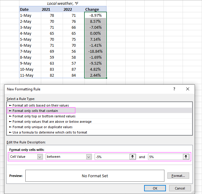
- Click the Format… button, and then choose the Fill or/and Font color you want.
- Click OK twice to close both dialog windows and your conditional formatting is done!

Excel conditional formatting based on another cell
In the previous examples, we highlighted cells based on "hardcoded" values. However, in some cases it makes more sense to base your condition on a value in another cell. The advantage of this approach is that irrespective of how the cell value changes in future, your formatting will adjust automatically to respond to the change.
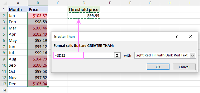
As an example, let's highlight prices in column B that are greater than the threshold price in cell D2. To accomplish this, the steps are:
- Click Conditional formatting> Highlight Cells Rules > Greater Than…
- In the dialog box that pops up, place the cursor in the text box on the left (or click the Collapse Dialog icon), and select cell D2.
- When done, click OK.
As a result, all the prices higher than the value in D2 will get highlighted with the selected color:
That is the simplest case of conditional formatting based on another cell. More complex scenarios may require the use of formulas. And you can find several examples of such formulas along with the step-by-step instructions here:
Apply multiple conditional formatting rules to same cells
When using conditional formats in Excel, you are not limited to only one rule per cell. You can apply as many rules as your business logic requires.
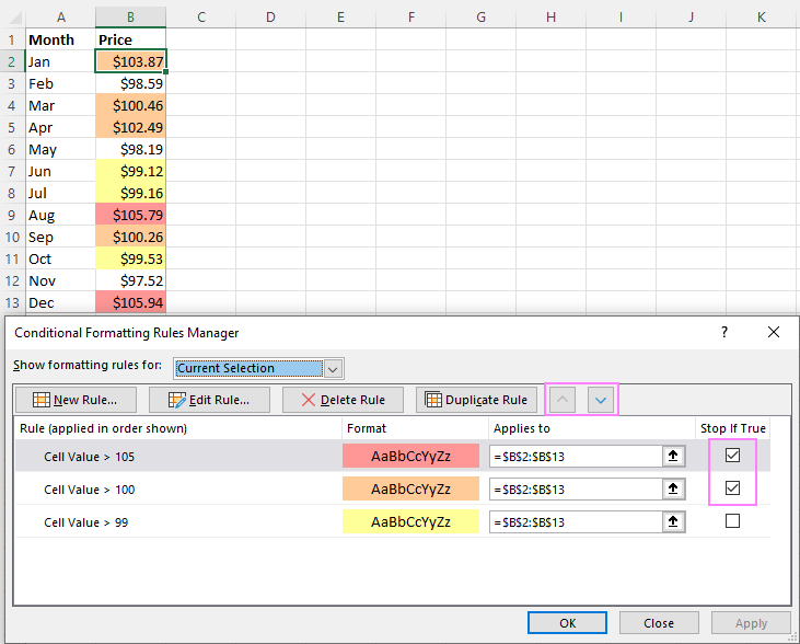
For example, you can create 3 rules to highlight prices higher than $105 in red, higher than $100 in orange, and higher than $99 in yellow. For the rules to work correctly, you need to arrange them in the right order. If the "greater than 99" rule is placed first, then only the yellow formatting will be applied because the other two rules won't have a chance to be triggered - obviously, any number that is higher than 100 or 105 is also higher than 99 :)
To re-arrange the rules, this is what you need to do:
- Select any cell in your dataset covered by the rules.
- Open the Rules Manager by clicking Conditional Formatting > Manage Rules…
- Click the rule that needs to be applied first, and then use the upward arrow to move it to top. Do the same for the second-in-priority rule.
- Select the Stop If True check box next to all but the last rule because you do not want the subsequent rules to be applied when the prior condition is met.
What is Stop if True in Excel conditional formatting?
The Stop If True option in conditional formatting prevents Excel from processing other rules when a condition in the current rule is met. In other words, if two or more rules are set for the same cell and Stop if True is enabled for the first rule, the subsequent rules are disregarded after the first rule is activated.
In the example above, we have already used this option to ignore subsequent rules when the first-in-priority rule applies. That usage is quite evident. And here are another couple of examples where the use of the Stop If True function is not so obvious but extremely helpful:
How to edit Excel conditional formatting rules
To make some changes to an existing rule, proceed in this way:
- Select any cell to which the rule applies and click Conditional Formatting > Manage Rules…
- In the Rules Manager dialog box, click the rule you want to modify, and then click the Edit Rule… button.
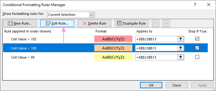
- In the Edit Formatting Rule dialog window, make the required changes and click OK to save the edits.
That dialog window looks very similar to the New Formatting Rule dialog box used for creating a new rule, so you won't have any difficulties with it.
Tip. If you don't see the rule you want to edit, then select This Worksheet from the Show formatting rules for drop-down list at the top of the Rules Manager dialog box. This will display the list of all the rules in your worksheet.
How to copy Excel conditional formatting
To apply a conditional format you've created earlier to other data, you won't need to re-create a similar rule from scratch. Simply use Format Painter to copy the existing conditional formatting rule(s) to another data set. Here's how:
- Click any cell with the formatting you want to copy.
- Click Home > Format Painter. This will change the mouse pointer to a paintbrush.
Tip. To copy the formatting to multiple non-contiguous cells or ranges, double-click Format Painter.
- To paste the copied formatting, click on the first cell and drag the paintbrush down to the last cell in the range you want to format.

- When done, press Esc to stop using the paintbrush.
- Select any cell in your new dataset, open the Rules Manager and check the copied rule(s).
Note. If the copied conditional formatting uses a formula, you may need to adjust cell references in the formula after copying the rule.
How to delete conditional formatting rules
I've saved the easiest part for last :) To delete a rule, you can either:
- Open the Conditional Formatting Rules Manager, select the rule and click the Delete Rule button.

- Select the range of cells, click Conditional Formatting > Clear Rules and choose the option that fits your needs.

This is how you do conditional formatting in Excel. Hopefully, these very simple rules we created were helpful to get a grasp of the basics. Below, you can find a few more tutorials that can help you understand the inner mechanics and expand conditional formatting in your spreadsheets far beyond its traditional uses.
Practice workbook for download
Excel conditional formatting - examples (.xlsx file)
 by
by
318 comments
Hi,
I am trying to find a way to get excel to conditionally format nonconsecutive cells if the values don't equal each other in all the specific cells but ignore that cell if it equals 0 and still do the comparison.
Hi! Your description of the rules for conditional formatting is not very clear. However, in the Conditional Formatting > Manage Rules > Edit Rule > “Applies to” field, you can specify all cells and ranges to which you want to apply the conditional formatting rule. For example: $A$1:$A$2,$A$4,$A$7:$A$10. You can also select these non-contiguous cells when creating conditional formatting.
For more information, please visit: Excel conditional formatting formulas based on another cell and How to select multiple cells in Excel: non-adjacent, visible, with data.
Hello
Is it possible to do the following - I have two rules over the same set of cells. The rules are no mutually exclusive. I'd like the first rule to change background colour and the second rule to change font colour - this way I can see when none/one (for each of the rules)/both conditions are met.
However when I set it up - I see that one rule overwrites the other (e g the font colour also covers the background with white, no the background visible from the other rule).
Is it possible to have one rule only change font colour and not background, and another rule to only modify background colour but not font?
Thanks
Actually, I managed to do it myself. Had to got into the "Font colour" rules and make sure the background is set to No colour (by pressing Clear)
I have an array of numbers by year (column) D5:H10, the year is in row 4. I would like to highlight a entire column if the year for that column = the value in a cell that the user enters at the top - cell C2. It seems simple enough, but I'm having trouble.
I tried D$4=$C$2 applied to D4:D10
Hello Sharon!
Select the range D4:H10 and create a conditional formatting rule for it:
=D$4=$C$2
Here is the article that may be helpful to you: Excel: Change the row color based on cell value.
Hi,
I have a monthly dashboard with Plan vs Actual in Horizontal rows, and I am using a conditional formatting red or green based on Plan vs actual, but when I copy the format to the posterior cells, it keeps the original (plan) as reference.
How can I do a conditional formatting for each cell?
Thanks,
Alex
Hi Alex!
Pay attention to the following paragraph of the article above: Copy conditional formatting. If this is not what you wanted, please let me know and I will try to help you.
Sir, at present I am facing these two problems. Please help me.
1) I want to know one thing that when we are writing the formulas in the cell then those formulas are visible or going in the formula bar. I want to write that formula or formulas by VBA to solve the problem. How is it possible? If you give a detailed guide, it will be very helpful. For example, I am doing Date of Retirement calculation with EOMONTH or I am writing a specific formula in a cell to calculate Present Age. I want to run these formulas with VBA. How to do? That means, I will write date of birth in one cell and present age in another cell and Retirement Date will be written in another cell simultaneously/automatically.
2) In those cells that cannot be duplicate entries, how can it be solved by conditional formatting? Means, I wrote the ID code in a cell, in the next case when entering that ID, a massage will show that this ID has been entered. It would be very helpful to know in detail how it can be solved.
Hi! Your first question can be solved without VBA with the help of this guide: How to calculate age in Excel from birthday.
The answer to your second question can be found here: Data validation to allow only unique entries and disallow duplicates.
Hi,
I am trying to make a conditional format based on a range of numbers.
For example, if the cell has a value outside of 15-20%, say with a range of 10-14% I want it to show red but if it falls into the range, such as 16-18% I want it to display green. Is it possible to do this based off of a range value in the cell or does it have to be a single number in the cell for the format to work?
Also the value I would be putting in the cells would be 10-14% and 16-18% in the above examples.
Thank you
Hi! For each color, create a separate conditional formatting rule as described in the article above. To do this, write a single number in the cell. 16-18% is text.
You can find useful information in this article: Change background color based on cell value.
I have twelve rules that format some cells based on conditions of some other cell which works just fine. When I copy the formatting to a new sheet in the same workbook, the rule copied adds the sheet name of the source. The find and replace formulas does not edit conditional rule formulae.
I have to manually delete the 'sheetname'! from each of the 12 copied formulae.
I'm pretty sure it's not possible, but maybe you guys know a way around; Is there any way to do partial formatting of a cell, that's the result of a formula?
I have a cell that's the output of a formula, which is a text string, and I want to underline the first word/first 10 characters of that string.
Hi! You cannot format part of a cell using conditional formatting.
Is there a way to highlight all cells that are not formula (ie. hardcoded) to show where formulas in a range have been written over?
Hi! We have a tool that can solve your task in a couple of clicks - Select by Value & Color tool. Use Select Special Cells - Select cells containing formulas option. The tool is included in the Ultimate Suite for Excel and can be used in a free trial to see how it works.
Hello, I'm trying to determine how I can conditionally format a range of months based off of the Effective and expiration month dates, as well as the Start month.
On the first example, the Start Month is Jan, that would be the first month cell to highlight, followed by the duration of months (differenc between Jan 2023 and March 2024 (14 months).
In the next example, Start month is May, followed by a duration of 16 months ending in Sept (aligned with the Sept expiration date).
Effective date will always be a prior date to the Expiration Date; duration can be anywhere from 6 months to 29 months; Start month will either be same month as effective date or the following month.
Appreciate you taking the time to review!
EffectiveDate ExpirationDate StartMonth Jan Feb Mar Apr May Jun Jul Aug Sep Oct Nov Dec Jan Feb Mar Apr May Jun Jul
1/1/2023 3/1/2024 Jan (JAN through March cells would be highlighted)
4/1/2023 7/15/2024 May (MAY through July cells would be highlighted)
Hi! You can find the examples and detailed instructions here: Excel conditional formatting for dates & time: formulas and rules.
I've already applied CF to a row on selected cells, this is based on a drop down "Yes" in one cell. This then changes the selected cells to change colour, however I want to expand the cell ranges from the CF Rule but I cannot work out how to do this. I've tried copy/Special paste and the paint brush and this just copies the text, colour of the already CF cells.
Please help :-)
Hi! To expand the range of conditional formatting cells, use rule editing as recommended in the article above.
Hi,
I've tried this method:
Click the first cell out of cell range which has the format
Double click the paint brush as it has multiple columns, which are not in order
Highlight the cells I want to include in the format, but it will then just colour code the entire range, this is without selecting the drop down option on row 2 to have that format..
I have told you how to do things correctly. Also note that copying the format changes the references in the conditional formatting formula. Read more: Relative and absolute cell references in Excel conditional formatting.
Hi, I am trying to highlight all the zero values in a row after a certain number
Example I have:
100 in A1 is the total which is made of
25 (A2), 0 (A3), 20, 15, 0, 40, 0, 0 (A9)
So I want to highlight the 0 values after 40 in cell A7.
The numbers something don't add exactly to 100, so I must use some formula which say highlight if value is zero.
Thanks in advance
Hi! In the conditional formatting formula, you must specify the exact cell by which the conditional formatting is done. In your case this is not possible.
I am wanting to figure out how to duplicate conditional formatting down 15 rows in a column. An example of the first row will be =$L$7>$D$7 (turns L7 red). Is there a way to drag this down to row 8, to auto create the same conditional formatting - =$L$8>$D$8 (turns L8 red) without having to create the conditional formatting manually for cell in the column?
Hi! Apply the formula =L1>D1 to your desired range of cells in column L as described in the article above.
I tried this multiple times and multiple ways. It never created another rule and all of the cells I copied to relied on the original cell's rule to determine the color. Ultimately I had to manually create a rule for each cell/row.
Hello Sir!
I am trying to highlight the whole row based on the first word I insert, for example:
Region 1 = red, Region 2 = blue;
So, when I type region 1, the column and its row will become red.
Do you have a formula that I could use to do this? or do you have the guideline to do this in conditional formatting rules manager?
Hi! Maybe this article will be helpful: Change the row color based on cell value.
Hello! I am trying to highlight cells based on if another cell has a date entered in it (cell in column "I" will need to change color once the corresponding cells in columns L, M, and N (each need to change individually). I do this to have an easy visual que that a sub-task has been completed. Cells in columns L, M, and N will be given dates once reports are issued/tasks completed - cells in L will get dates first, then M, and then N. Each row is a different item, and once the cells from L, M, and N are given dates, I need that row's "I" cell to change color. I was doing it by the NOT ISBLANK function, but then it would multiply/separate out when you open up rules, so adding a new one was difficult. I started out with 3 rules, and then they altered themselves and ended up showing up as twenty some, or more, different rules.
So I guess two questions - do you have a formula that I could use to do this? And how do you keep rules from multiplying/modifying themselves?
Thanks!
Hi! If I understand your task correctly, try the following conditional formatting formula:
=AND(ISNUMBER(L1:N1))
THanks for your well described help on this topic. Can the output be text rather than colour? i.e. if something needs action it would display action rather than red?
Hi! Conditional formatting can only change the format of a cell, not its value. To change the value, use Excel formulas.
Hi,
I am wanting to create a conditional formatting rule that highlights cells D8 and E8 if any cell between F8 and V8 have a value of 1-99. Is this possible?
Thanks in advance! I’ve tried lots of things but can’t get it to work.
Hi! Please try the following conditional formatting formula:
=SUM((F8:V8>0)*(F8:V8<100))>0
I appreciate the help. I'm not sure if you can help further. But when I have applied these rules and reviewed the section you suggested the formulas are highlighting date 8/1/23 yellow and 7/15/23 & 7/17/23 red even though they have not yet passed.
I think you didn't read this article very carefully. If the date is less than today, =$B2
Hey!
So, I am trying to set up a conditional formatting function to highlight cells greater than 130 in each row. However, once the first cell to reach 130 in the row is highlighted, I do not want the following numbers to be highlighted (since the numbers just increase).
I tried using the in-between function but that would give me a range greater than 30 for some rows and simply is not working for the spread I am using.
Is there a specific function for this in conditional formatting?
Hi! If I understand you correctly, to select only the first value greater than 130, select row 2 and create a conditional formatting rule:
=COUNTIF($A$2:A2,">130")=1
You can learn more about COUNTIF in this article: Excel COUNTIF function examples. Hope this is what you need.
Trying to find a conditional format solution to a stock available v continuous daily demand for a production week
As you may guess starting stock in the first day of the week maybe 100, but on each day of the week the stock that is to be consumed each day will run out on a particular day, question how can I highlight what day the stock will run out on , as I will have multiple rows of parts to apply this too, the idea is to plan production based upon run out day
Can you help I was thinking each cell will need some kind of subtraction referencing the row stock level
Hi! To calculate how many days' supply is enough, divide the beginning supply by the daily consumption. It is not possible to give more detailed advice without seeing your data.
Hello!
I find that in some files the conditional formatting "disappears" from one use to the next. I set it, it's working fine. And when I go back to the file another time, I have to set it again. In other files it's still there. I cannot work out why one would be different from the other. Is it to do with other settings in the individual files?
Thanks,
Manuela