The tutorial explains how to use COUNTIFS and COUNTIF formulas with multiple criteria in Excel based on AND as well as OR logic. You will find a number of examples for different data types - numbers, dates, text, wildcard characters, non-blank cells and more.
Of all Excel functions, COUNTIFS and COUNTIF are probably most often mixed up because they look very much alike and both are purposed for counting cells based on the specified criteria.
The difference is that COUNTIF is designed for counting cells with a single condition in one range, whereas COUNTIFS can evaluate different criteria in the same or in different ranges. The aim of this tutorial is to demonstrate different approaches and help you choose the most efficient formula for each particular task.
Excel COUNTIFS function - syntax and usage
The Excel COUNTIFS function counts cells across multiple ranges based on one or several conditions. The function is available in Excel 365, 2021, 2019, 2016, 2013, Excel 2010, and Excel 2007, so you can use the below examples in any Excel version.
COUNTIFS syntax
The syntax of the COUNTIFS function is as follows:
- criteria_range1 (required) - defines the first range to which the first condition (criteria1) shall be applied.
- criteria1 (required) - sets the condition in the form of a number, cell reference, text string, expression or another Excel function. The criteria defines which cells shall be counted and can be expressed as 10, "<=32", A6, "sweets".
- [criteria_range2, criteria2]… (optional) - these are additional ranges and their associated criteria. You can specify up to 127 range/criteria pairs in your formulas.
In fact, you don't have to remember the syntax of the COUNTIF function by heart. Microsoft Excel will display the function's arguments as soon as you start typing; the argument you are entering at the moment is highlighted in bold.

Excel COUNTIFS - things to remember!
- You can use the COUNTIFS function in Excel to count cells in a single range with a single condition as well as in multiple ranges with multiple conditions. If the latter, only those cells that meet all of the specified conditions are counted.
- Each additional range must have the same number of rows and columns as the first range (criteria_range1 argument).
- Both contiguous and non-contiguous ranges are allowed.
- If the criteria is a reference to an empty cell, the COUNTIFS function treats it as a zero value (0).
- You can use the wildcard characters in criteria - asterisk (*) and question mark (?). See this example for full details.
How to use COUNTIFS and COUNTIF with multiple criteria in Excel
Below you will find a number of formula examples that demonstrate how to use the COUNTIFS and COUNTIF functions in Excel to evaluate multiple conditions.
How to count cells with multiple criteria (AND logic)
This scenario is the easiest one, since the COUNTIFS function in Excel is designed to count only those cells for which all of the specified conditions are TRUE. We call it the AND logic, because Excel's AND function works this way.
Formula 1. COUNTIFS formula with multiple criteria
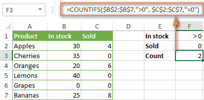
Suppose you have a product list like shown in the screenshot below. You want to get a count of items that are in stock (value in column B is greater than 0) but have not been sold yet (value is column C is equal to 0).
The task can be accomplished by using this formula:
=COUNTIFS(B2:B7,">0", C2:C7,"=0")
And the count is 2 ("Cherries" and "Lemons"):
Formula 2. COUNTIFS formula with two criteria
When you want to count items with identical criteria, you still need to supply each criteria_range / criteria pair individually.
For example, here's the right formula to count items that have 0 both in column B and column C:
=COUNTIFS($B$2:$B$7,"=0", $C$2:$C$7,"=0")
This COUNTIFS formula returns 1 because only "Grapes" have "0" value in both columns.
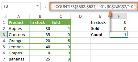
Using a simpler formula with a single criteria_range like COUNTIFS(B2:C7,"=0") would yield a different result - the total count of cells in the range B2:C7 containing a zero (which is 4 in this example).
How to count cells with multiple criteria (OR logic)
As you have seen in the above examples, counting cells that meet all of the specified criteria is easy because the COUNTIFS function is designed to work this way.
But what if you want to count cells for which at least one of the specified conditions is TRUE, i.e. based on the OR logic? Overall, there are two ways to do this - by adding up several COUNTIF formulas or using a SUM COUNTIFS formula with an array constant.
Formula 1. Add up two or more COUNTIF or COUNITFS formulas
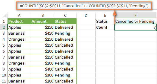
In the table below, supposing you want to count orders with the "Cancelled" and "Pending" status. To have it doen, you can simply write 2 regular Countif formulas and add up the results:
=COUNTIF($C$2:$C$11,"Cancelled") + COUNTIF($C$2:$C$11,"Pending")
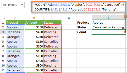
In case each of the functions is supposed to evaluate more than one condition, use COUNTIFS instead of COUNTIF. For example, to get the count of "Cancelled" and "Pending" orders for "Apples" use this formula:
=COUNTIFS($A$2:$A$11, "Apples", $C$2:$C$11,"Cancelled") + COUNTIFS($A$2:$A$11, "Apples", $C$2:$C$11,"Pending")
Formula 2. SUM COUNTIFS with an array constant
In situations when you have to evaluate a lot of criteria, the above approach is not the best way to go because your formula would grow too big in size. To perform the same calculations in a more compact formula, list all of your criteria in an array constant, and supply that array to the criteria argument of the COUNTIFS function. To get the total count, embed COUNTIFS inside the SUM function, like this:
In our sample table, to count orders with the status "Cancelled" or "Pending" or "In transit", the formula would go as follows:
=SUM(COUNTIFS($C$2:$C$11, {"cancelled", "pending", "in transit"}))
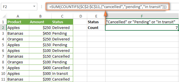
In a similar manner, you can count cells based on two or more criteria_range / criteria pairs. For instance, to get the number of "Apples" orders that are "Cancelled" or "Pending" or "In transit", use this formula:
=SUM(COUNTIFS($A$2:$A$11,"apples",$C$2:$C$11,{"cancelled","pending","in transit"}))

You can find a few more ways to count cells with OR logic in this tutorial: Excel COUNTIF and COUNTIFS with OR conditions.
How to count numbers between 2 specified numbers
By and large, COUNTIFS formulas for numbers fall into 2 categories - based on several conditions (explained in the above examples) and between the two values you specify. The latter can be accomplished in two ways - by using the COUNTIFS function or by subtracting one COUNTIF from another.
Formula 1. COUNTIFS to count cells between two numbers
To find out how many numbers between 5 and 10 (not including 5 and 10) are contained in cells C2 through C10, use this formula:
=COUNTIFS(C2:C10,">5", C2:C10,"<10")
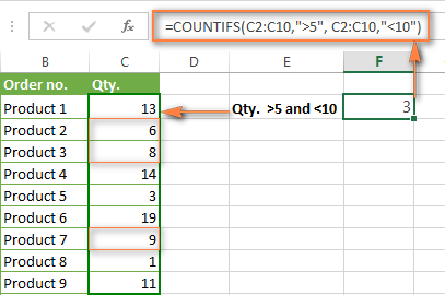
To include 5 and 10 in the count, use the "greater than or equal to" and "less than or equal to" operators:
=COUNTIFS(B2:B10,">=5", B2:B10,"<=10")
Formula 2. COUNTIF formulas to count numbers between X and Y
The same result can be achieved by subtracting one Countif formula from another. The first one counts how many numbers are greater than the lower bound value (5 in this example). The second formula returns the count of numbers that are greater than the upper bound value (10 in this case). The difference between the first and second number is the result you are looking for.
- =COUNTIF(C2:C10,">5")-COUNTIF(C2:C10,">=10") - counts how many numbers greater than 5 and less than 10 are in the range C2:C10. This formula will return the same count as shown in the screenshot above.
- =COUNTIF(C2:C10, ">=5")-COUNTIF(C2:C10, ">10") - the formula counts how many numbers between 5 and 10 are in the range C2:C10, including 5 and 10.
How to use cell references in COUNTIFS formulas
When using logical operators such as ">", "<", "<=" or ">=" together with cell references in your Excel COUNTIFS formulas, remember to enclose the operator in "double quotes" and
add an ampersand (&) before a cell reference to construct a text string.
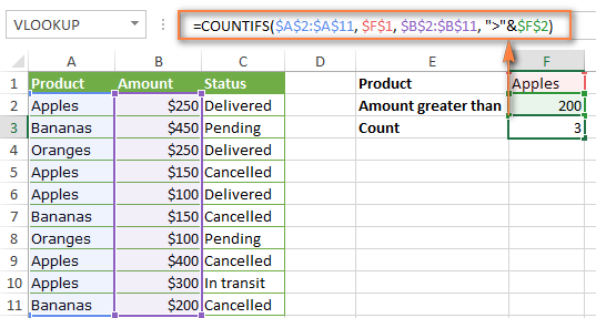
In a sample dataset below, let's count "Apples" orders with amount greater than $200. With criteria_range1 in cells A2:A11 and criteria_range2 in B2:B11, you can use this formula:
=COUNTIFS($A$2:$A$11, "Apples", $B$2:$B$11, ">200")
Or, you can input your criteria values in certain cells, say F1 and F2, and reference those cells in your formula:
=COUNTIFS($A$2:$A$11, $F$1, $B$2:$B$11, ">"&$F$2)
Please notice the use of absolute cell references both in the criteria and criteria_range arguments, which prevents the formula from being broken when copied to other cells.
For more information about the use of an ampersand in COUNTIF and COUNTIFS formulas, please see Excel COUNTIF - frequently asked questions.
How to use COUNTIFS with wildcard characters
In Excel COUNTIFS formulas, you can use the following wildcard characters:
- Question mark (?) - matches any single character, use it to count cells starting and/or ending with certain characters.
- Asterisk (*) - matches any sequence of characters, you use it to count cells containing a specified word or a character(s) as part of the cell's contents.
Tip. If you want to count cells with an actual question mark or asterisk, type a tilde (~) before an asterisk or question mark.
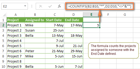
Now let's see how you can use a wildcard char in real-life COUNTIFS formulas in Excel. Suppose, you have a list of projects in column A. You wish to know how many projects are already assigned to someone, i.e. have any name in column B. And because we are learning how to use the COUNTIFS function with multiple criteria, let's add a second condition - the End Date in column D should also be set.
Here is the formula that works a treat:
=COUNTIFS(B2:B10,"*",D2:D10,"<>"&""))
Please note, you cannot use a wildcard character in the 2nd criteria because you have dates rather that text values in column D. That is why, you use the criteria that finds non-blank cells: "<>"&""
COUNTIFS and COUNTIF with multiple criteria for dates
The COUNTIFS and COUNTIF formulas you use for dates are very much similar to the above formulas for numbers.
Example 1. Count dates in a specific date range
To count the dates that fall in a certain date range, you can also use either a COUNTIFS formula with two criteria or a combination of two COUNTIF functions.
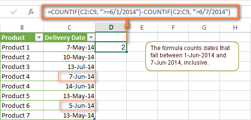
For example, the following formulas count the number of dates in cells C2 through C10 that fall between 1-Jun-2014 and 7-Jun-2014, inclusive:
=COUNTIFS(C2:C9, ">=6/1/2014", C2:C9, "<=6/7/2014")
=COUNTIF(C2:C9, ">=6/1/2014") - COUNTIF(C2:C9, ">6/7/2014")
Example 2. Count dates with multiple conditions
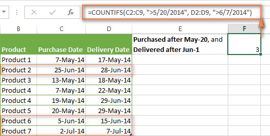
In the same manner, you can use a COUNTIFS formula to count the number of dates in different columns that meet 2 or more conditions. For instance, the below formula will find out how many products were purchased after the 20th of May and delivered after the 1st of June:
=COUNTIFS(C2:C9, ">5/1/2014", D2:D9, ">6/7/2014")
Example 3. Count dates with multiple conditions based on the current date
You can use Excel's TODAY() function in combination with COUNTIF to count dates based on the current date.
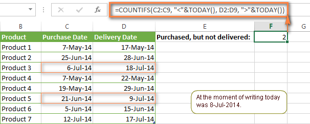
For example, the following COUNTIF formula with two ranges and two criteria will tell you how many products have already been purchased but not delivered yet.
=COUNTIFS(C2:C9, "<"&TODAY(), D2:D9, ">"&TODAY())
This formula allows for many possible variations. For instance, you can tweak it to count how many products were purchased more than a week ago and are not delivered yet:
=COUNTIFS(C2:C9, "<="&TODAY()-7, D2:D9, ">"&TODAY())
This is how you count cells with multiple criteria in Excel. I hope you will find these examples helpful. Anyway, I thank you for reading and hope to see you on our blog next week!
 by
by
599 comments
Hello, I have a file and I am not sure if the CountIFS function is the one to use. I have 4 columns containing either Yes, No or Pending and I want to count how many the "Yes" appears in at least 3, at least 2 and at least 1 column, separately for each case. I have used the COUNTIF function to count all the Yes cells in all 4 columns, but I am struggling with the function to count in not all 4 columns. Any help will be appreciated :)
Hi! COUNTIFS alone can’t do this, because you’re counting per row across multiple columns (not down a single column).
You need to count YES per row, then summarize. Reliable solutions depending on your Excel version.
Excel365/2021 formula:
=SUM(--(BYROW(A2:D100, LAMBDA(r, COUNTIF(r,"Yes")>=1))))
where data in A2:D100, each cell contains: Yes / No / Pending.
Read more: Excel LAMBDA function: how to write, calculate and use.
Array formula in older Excel versions:
=SUM(--(MMULT(--(A2:D100="Yes"),{1;1;1;1})>=1))
Use Ctrl+Shift+Enter if required.
I need help with a formula for tallying up texts. I need to total up the number of complaints in a certain neighborhood, but I need to subtract duplicate complaints. Right now, I have the neighborhoods in a column (A), and the next column (B) has the following examples of types of data: Duplicate, Closed, date, etc. I need to total up the specific neighborhoods in A but subtract any in column B that has duplicate and closed. I've tried =COUNTIF(A:A,"NORTHSIDE")-(COUNTIF(B:B,"DUPLICATE")+COUNTIF(B:B,"CLOSED")) but the counts are still off. It works if there's only 1 subtracted category.
Thanks!
Hello Elizabeth!
Based on your description, it is hard to completely understand your task. However, I’ll try to guess and offer you the following formula:
=COUNTIF(A:A,"NORTHSIDE")-(COUNTIFS(A:A,"NORTHSIDE",B:B,"DUPLICATE")+COUNTIFS(A:A,"NORTHSIDE",B:B,"CLOSED"))
Hi Alex,
I'm having some trouble trying to figure out the correct COUNTIF formula for what I want to do. For instance, I have a Column F that contains years 2021 through 2025 and Column H that contains the status of either "Awarded", "Cancelled", "In Progress", etc.
I need a formula that gives me the total number of cells that contain both 2021 AND Awarded or 2021 AND Cancelled, etc (both criteria in this case must be met).
The COUNTIF formula I tried using counts all rows that contain 2021 OR Awarded. So instead of ending up with a total # of 302 cells that contain both 2021 and Awarded, I end up with a total # of 1902 because the formula is counting 2021 or Awarded.
I've tried variations of the formula below but I keep getting 1902 total Awarded back when there are only 300 Awarded in 2021, the rest are either Cancelled or In Progress.
=COUNTIFS($H$13:$H$2000,"Awarded", $F$13:$F$2000, "2021")
Please help!
Hello Anna!
If I understand your task correctly, all the necessary information is in the article above.
=COUNTIFS($H$13:$H$2000,"Awarded", $F$13:$F$2000, "2021")+COUNTIFS($H$13:$H$2000,"Cancelled", $F$13:$F$2000, "2021")
Hi,
I am trying to count how many ROWS have a date greater that 2025-01-01 AND has a specific text. every combination of countifs and countif is not giving me the correct information. Is there a formula for this?
use COUNTIFS
I have a file where Column E Contains contains a name. I want a formula to Search column E and if the name equals "Vacant" then I want cell F4 to equal "Red", if it contains the partial word "Pending" then I was cell F4 to equal "Yellow" for all other entries I want F4 to eqaul "Green"
The formula I have tried using is =IF(E4="","",IF(E4="Vacant", "Red", IF(COUNTIF(E4,"Pending"),"Yellow","Green"))) but its not picking up the "Pending"
I'm sure its something simple..thanks
=IF(E4="VACANT","RED",IF(E4="PENDING","YELLOW"),"GREEN"))
Hello Breda!
To find a partial match, use this expression:
COUNTIF(E4,"*Pending*")
Read more: Excel IF statement for partial text match (wildcard).
Hello!
for example, I've got 5 subjects here : Geography | History | Art | Science | Physics
I'd like to count number of students who pick specific subjects as their choices.
So in 2 cells, for example, if a student type 'Art' and 'Physics', no matter what's the order that student put, still count that combination as 1 (number shows on another cell).
Can I have a formula showing that please ?
Hello Ringo!
If I understand your task correctly, the following formula should work for you:
=FILTER(A2:A12,BYROW(FILTER(
(B2:E12="Physics")+(B2:E12="Art"),
(BYROW((B2:E12="Physics")+(B2:E12="Art"), LAMBDA(r, COUNT(r)>0)))
),LAMBDA(r,SUM(r)))>0)
This formula filters the range A2:A12 to return only the rows where at least one of the subjects in columns B2:E12 is either "Physics" or "Art".
FILTER(A2:A12, ...) filters the range A2:A12 based on the condition provided.
BYROW(FILTER((B2:E12="Physics") + (B2:E12="Art"), (BYROW((B2:E12="Physics")+(B2:E12="Art"), LAMBDA(r, COUNT(r)>0)))), LAMBDA(r, SUM(r)))>0 creates a condition to filter the rows:
(B2:E12="Physics")+(B2:E12="Art") creates a logical array where each cell is TRUE if it contains "Physics" or "Art", and FALSE otherwise.
I recommend reading this guide: Excel LAMBDA function: how to write, calculate and use.
FILTER(..., (BYROW((B2:E12="Physics")+(B2:E12="Art"), LAMBDA(r, COUNT(r)>0)))) filters this logical array to keep only the rows where at least one cell is TRUE.
BYROW(..., LAMBDA(r, SUM(r))) sums the TRUE values in each row, resulting in an array of row sums.
>0 checks if the sum of TRUE values in each row is greater than 0, indicating that the row contains at least one "Physics" or "Art".
That really helps !
Thanks so much Sir !
i have alarm list in individual sheets for each day in excel workbook, now i have a summary sheet where i need to count the closed and open alarms against each department for each day and display in the summary sheet against each date
Hi! You can create a separate COUNTIFS formula for each worksheet to count closed and open alarms against each department. Your information is not enough to recommend a formula to you.
You can also combine data from all worksheets on a single worksheet. Use any of the methods described in this guide: Consolidate data in Excel and merge multiple sheets into one worksheet.
Create a pivot table for this consolidated data and create all the necessary fields in it to calculate the values. Read more: How to use Pivot Tables in Excel.
In Excel 365, you can also group and summarize data using a PIVOTBY formula.
Greetings and thank you for the excellent tutorial! I wanted to ask, is there a way to set up a COUNTIFS formula that tabulates distinct individuals meeting one criteria on a specified sheet and also excludes a specific value under a different criteria? To clarify, I am attempting to tabulate employees assigned a specific role (e.g. TrainingManager, TrainingFacilitator, etc.) across the different working groups at each office on my company's campus, where a given individual may have the same role across multiple groups, and certain groups may have vacancies*. My workbook is divided into sheets corresponding to office (Office1, Office2, etc.) with each sheet organized as:
(A)Group# (B)LastName (C)FirstName (D)Email (E)Role
As individual COUNTIF statements these desired outputs seem fairly straightforward [e.g. =COUNTIF(Office1!$E:$E,"TrainingManager") to tabulate role assignments in one office]; my issue lies in crafting a COUNTIFS statement that totals a given value (e.g. TrainingManager) in Column E (Role) BUT only for distinct values in Column D (Email), AND excludes any cell in Column D whose value is "Vacant". Additionally, this needs to be on a separate Totals sheet in the workbook, as this is a shared worksheet that office managers at each location will be updating as roles are filled (for this reason, helper columns and pivot tables are not options I can pursue).
*[Example: In Office1, JaneDoe@ company.com is assigned TrainingManager for Groups 1, 3, and 5; Group 2's TrainingManager is Vacant, and JohnQPublic@ company.com is TrainingManager for Group 4. What would be the cleanest way to ensure the correct TrainingManager count on the Totals tab is 2?]
Hi! If I understand the question correctly, you want to count the number of unique values that match certain conditions. We have a special tutorial that can help to solve your problem: Count unique values with multiple criteria.
Based on your information, the formula might look something like this:
=IFERROR(ROWS(UNIQUE(FILTER(D:D,(E:E="TrainingManager")*(D:D<>"Vacant"),""))),0)
Greetings! That solved the issue handily- thank you so much!
I have the following formula that is not valid and I'm not sure what the problem is. I want to count the occurences of the value in cell B1 (Bob) in sheet week1!j35 thru week1!l35. The value week1 is in cell a3. Do I have to use INDIRECT? If I hard code week1 in the formula it works. Please help thanks.
=COUNTIF("'"&a3&"'!$J$35:"'"&a3&"'!$L$35,"*"&$B$1&"*")
Hello Bob!
If I understand your task correctly, you can find the answer to your question in this guide: COUNTIF with wildcard characters (partial match). Try this formula:
=COUNTIF($J$35:$L$35,"*"&A3&"*")
So I figured it out. This works =COUNTIF(INDIRECT("'"&A3&"'!$J$35"):INDIRECT("'"&A3&"'!$L$35"),"*"&$B$1&"*")
I have 60 alphabets in 60 columns in first row. In the second row, I have another 60 alphabets. I want to count the alphabets in first row that matches with alphabets in the second row at the same position. Please suggest.
Hi! To count the number of matches in two rows, you can use the SUMPRODUCT formula. If I understand your task correctly, the formula might look something like this:
=SUMPRODUCT(--(A1:Z1=A2:Z2))
Hi there,
so I'm trying to make a formula where I want to calculate hours in a timesheet.
Cells D13-D30 contain the activity.
Cells E13-E30 contain the hours worked.
I want the formula to check D13-D30 for A/L and then sum up the hours corresponding to those cells.
Is there a way I can do that?
I've tried a few versions, but couldn't come up with anything.
Thanks.
Hello Kathrin!
All the necessary information is in the article: Excel SUMIFS and SUMIF with multiple criteria – formula examples. If I understand your task correctly, the following formula should work for you:
=SUMIFS(E13:E30,D13:D30,"A")
I have a list of 3000 different names and I need to highlight all names that appear fewer than 8 times.
Hi! For the range A2:A3000, you can use a conditional formatting rule like this:
=COUNTIF($A$2:$A$3000,A2)<8
We have a special tutorial on this. Please see: How to highlight duplicate cells and rows in Excel.
Hi Sir,
Good day to you. I am trying to track stock price movements relative to its moving average ‘MA’, basically how many days it had stayed above the MA (before ‘going below’) and vice versa.
My column A2:A300 contains the dates (with A300 the most recent), B2:B300 the ‘closing price (for that day)’, and C2:C300 a ‘MA’. An example to illustrate what I wish to have please.
P > MA ‘dates’
Price B300 is 100, MA C300 is 98 Y today
B299 is 95 C299 is 91 Y day-before
B298 is 60 C298 is 70 N 2 day before
B297 is 85 C297 is 72 Y and so on
I would like to have a formula output like “XaMAby2D” (which is cross above MA for past 2 days) for above instance (and if converse is true, “XbMAby2D”). I am unsure if I should post here as I think COUNTIF is regardless of the order it appears as long as it is within a ‘date range’ but here I need to ‘count backwards’ the number of days from today it stays above / below the MA (that is start from cell 300 followed by 299 and so on). Ignore Price=MA please.
Could kindly advise please?
Much obliged. Wishing you and loved ones health and bliss.
Sincerely,
Hi! If I understand your task correctly, write this formula in cell C3 and then copy it down along the column:
=IF(B3>C3,COUNT($B$2:B3) - IFERROR(XMATCH(B3>C3,$B$2:B2<$C$2:C2,0,-1),0),0)
XMATCH function searches a column to find the nearest value that does not satisfy the IF condition.
I hope my advice will help you solve your task.
Hello
I have a spreadsheet where on a separate tab I need excel to add up the figures in column M if the month in column D is October, then again the figures in column M if the month in column D is November so that on the separate tab I send up with:
October £***
November £***
December £*** etc - all based on the information on the first spreadsheet.
Does that make sense? Can someone help??
Hello!
You can calculate the sum of the condition by using the SUMIF function. For example:
=SUMIF(D2:D100,"October",M2:M100)
If column D contains dates rather than the name of the month, use the SUMIFS function. You can find the examples and detailed instructions here: Excel SUMIFS and SUMIF with multiple criteria – formula examples.
=SUMIFS(M2:M100,D2:D100,">="&DATE(2024,10,1),D2:D100,"<="&DATE(2024,10,31))
Instead of using the DATE function in a formula, you can use a reference to a cell with a date.
You can also use the SUMPRODUCT function as described in these instructions: Excel SUMPRODUCT function with multiple criteria. To get the month number, use the MONTH function. For example:
=SUMPRODUCT(M2:M100*(MONTH(D2:D100)=10))
That is SO helpful - thank you!
How do I get that information from one sheet to another? My data is on one tab - and I need the totals to be on a separate tab.
Sorry - I feel I should know that!!
Hi! If I understand your task correctly, you can use references to another sheet in the formula. I recommend reading this guide: Excel reference to another sheet or workbook (external reference).
I have a student who created a spreadsheet based on a questionaire. She wants to count all the 5s in each cell when there are multiple numbers in that cell. Is there a way to do that? Does she have to redo the spreadsheet so only one number is i each cell?
So there is a range of cells B2:B8
B2 might have this data 1,2,5,6
B3 contains 3,5,7,9
B4 contains 1,3,6,7
B5 contains 1,2,6,7
B6 contains 1,3,5,7
B7 contains 2,4,5,7
B8 contains 3,6,7
Hello Irene!
If you want to find the sum of numbers within a single cell in Excel, you can use a combination of SUMPRODUCT and TEXTSPLIT functions.
=SUMPRODUCT(--TEXTSPLIT(B2,,","))
You can also extract all characters sequentially from the text using MID function. Using a mathematical operation and IFERROR function, determine all numbers and sum them with SUMPRODUCT.
=SUMPRODUCT(IFERROR(MID(B2,ROW(INDIRECT("1:"&LEN(B2))),1)*1,0))
If TEXTSPLIT isn't available, also you can use this approach:
Split the values manually:
Use Text to Columns feature found under the Data tab and split by comma delimiter.
Sum the values: Use the SUM function.
I have the following formula set- IF(COUNTIFS(N4,"EXP",P4,"EXP",R4,"EXP"),"EXP","") and want to add a second option e.g. IF(COUNTIFS(N4,"EXP",P4,"EXP",R4,"EXP"),"EXP",""),countifs(N4,"GDS",P4,"GDS",R4,"GDS"),"GDS")). I need it to return based on the criteria being met in all three columns. I've managed to achieve this with the one (first formula) using a couple of different types of formula but cannot get it to work with the second part. Can anyone help?
Hello Nic!
If I understand your task correctly, you want to check values in three cells.
The formula might look like this:
=IF(COUNTIFS(N4,"EXP",P4,"EXP",R4,"EXP"),"EXP", IF(COUNTIFS(N4,"GDS",P4,"GDS",R4,"GDS"),"GDS",""))
In such cases, it is a common practice to use the nested IF formula as it is described in this guide: Nested IF in Excel – formula with multiple conditions. For example:
=IF(AND(N4="EXP",P4="EXP",R4="EXP"),"EXP", IF(AND(N4="GDS",P4="GDS",R4="GDS"),"GDS",""))
Hope this is what you need.
Hi Alexander, that is exactly what I needed! Thank you very much, I've been going round in circles!
I have countcellsbycolor formula set up. Is there a way I can use this in combination with COUNTIFS?
For example, count if a range of cells is a particular color AND if a range of cells has a specific letter entered into it.
something like =COUNTIFS(F10:F9999,"Y",=countcellsbycolor(K10:K10057,K1))
Hello Sarah!
To count the number of cells that contain a particular letter and are highlighted in a particular color, use the custom function GetCellColor and the SUMPRODUCT formula.
=SUMPRODUCT((GetCellColor(A2:A15)=49407) * (ISNUMBER(SEARCH("A";A2:A15))))
For more information, please read: How to find substring in Excel.
Read more about using GetCellColor function here: How to get cell color in Excel.
can I use countifs to count multiple occurrences of the same string in a single cell.
For instance
cell a1 contains "loan loan"
cell a2 contains "loan"
cell a3 contains "loan loan loan"
I want to see a count of 6.
Hello Anthony!
The answer to your question can be found in this guide: Count only specific words / text in a range. Try the following formula:
=SUMPRODUCT((LEN(A1:A3)-LEN(SUBSTITUTE(A1:A3, "loan","")))/LEN("loan"))
or
=(LEN(CONCAT(A1:A3)) - LEN(SUBSTITUTE(CONCAT(A1:A3),"loan",""))) / LEN("loan")
Hi, thank you for explanation for the use of countif and countifs for range of dates using ">5/1/2014" for example.
But can you give explanation about how to use this if i need to use the date entered in another cell, not in the formula it self.
For example : I have entered "1/1/2024" in one cell and "31/1/2024" in another one (3 months range). How to use both cell to in the countif/countifs formula?
It will ease the effort to mess with the formula again. Thank you.
Hello Edward!
You can use logical operators such as ">", "<", "<=" or ">=" together with cell references in your Excel COUNTIFS formulas. Remember to enclose the operator in "double quotes" and add concatenation operator (&) before a cell reference.
Cells may contain dates or numbers. For example:
=COUNTIFS(C2:C9,">="&A1,C2:C9,"<="&"B1")
Very helpful answer! It already solved my problem. Thank you very much.
Hi sir, please help to solve the below formula:
=Countifs(S4:S545,"0")
Hi! I can't guess what your problem is with this formula.