In this tutorial, you will find a handful of advanced formula examples that demonstrate how to use Excel's VLOOKUP and SUM or SUMIF functions to look up and sum values based on one or several criteria.
Are you trying to create a summary file in Excel that will identify all instances of one particular value, and then sum other values that are associated with those instances? Or, do you need to find all values in an array that meet the condition you specify and then sum the related values from another worksheet? Or maybe you are faced with a more concrete challenge, like looking through a table of your company invoices, identifying all invoices of a particular vendor, and then summing all the invoice values?
The tasks may vary, but the essence is the same - you want to look up and sum values with one or several criteria in Excel. What kind of values? Any numeric values. What sort of criteria? Any : ) Starting from a number or reference to a cell containing the right value, and ending with logical operators and results returned by Excel formulas.
So, does Microsoft Excel have any functionality that can help with the above tasks? Of course, it does! You can work out a solution by combining Excel's VLOOKUP or LOOKUP with SUM or SUMIF functions. The formula examples that follow below will help you understand how these Excel functions work and how to apply them to real data.
Please note, these are advanced examples that imply you are familiar with the general principles and syntax of the VLOOKUP function. If not, the first part of our VLOOKUP tutorial for beginners is certainly worth your attention - Excel VLOOKUP syntax and general usages.
Excel VLOOKUP and SUM - find the sum of matching values
If you work with numerical data in Excel, quite often you have not just to extract associated values from another table but also sum numbers in several columns or rows. To do this, you can use a combination of the SUM and VLOOKUP functions as demonstrated below.
Source data:
Suppose, you have a product list with sales figures for several months, a column per each month. The source data is on the sheet named Monthly Sales:

Now, you want to make a summary table with the total sales for each product.
The solution is to use an array in the 3rd parameter (col_index_num) of the Excel VLOOKUP function. Here is a generic formula:
As you see, we use an array constant in the third argument to perform several lookups within the same VLOOKUP formula in order to get the sum of values in columns 2,3 and 4.
And now, let's adjust this combination of VLOOKUP and SUM functions for our data to find the total of sales in columns B - M in the above table:
=SUM(VLOOKUP(B2, 'Monthly sales'! $A$2:$M$9, {2,3,4,5,6,7,8,9,10,11,12,13}, FALSE))
Important! Since you are building an array formula, be sure to hit Ctrl + Shift + Enter instead of a simple Enter keystroke when you finished typing. When you do this, Microsoft Excel encloses your formula in curly braces like this:
{=SUM(VLOOKUP(B2, 'Monthly sales'!$A$2:$M$9, {2,3,4,5,6,7,8,9,10,11,12,13}, FALSE))}
If you press the Enter key as usual, only the first value in the array will get processed, which will produce incorrect results.
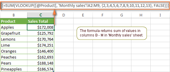
Tip. You may be curious why the formula displays [@Product] as the lookup value in the screenshot above. This is because I converted my data to table (Insert tab > Table). I find it very convenient to work with fully-functional Excel tables and their structured references. For example, when you type a formula into one cell, Excel automatically copies it across the entire column and in this way saves you a few precious seconds :)
As you see, using the VLOOKUP and SUM functions in Excel is easy. However, this is not the ideal solution, especially if you are working with big tables. The point is that using array formulas may adversely affect the workbook's performance since each value in the array makes a separate call of the VLOOKUP function. So, the more values you have in the array and the more array formulas you have in your workbook, the slower Excel works.
You can bypass this problem by using a combination of the INDEX and MATCH functions instead of SUM and VLOOKUP, and I will show you a few formula examples in the next article.
Download this VLOOKUP and SUM sample
How to perform other calculations with Excel VLOOKUP function
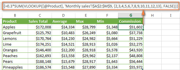
A moment ago we discussed an example of how you can extract values from several columns in the lookup table and calculate the sum of those values. In the same fashion, you can perform other mathematical calculations with the results returned by the VLOOKUP function. Here are a few formula examples:
| Operation | Formula example | Description |
|---|---|---|
| Calculate average | {=AVERAGE(VLOOKUP(A2, 'Lookup Table'$A$2:$D$10, {2,3,4}, FALSE))} | The formula searches for the value of cell A2 in 'Lookup table' and calculates the average of values in columns B,C and D in the same row. |
| Find maximum value | {=MAX(VLOOKUP(A2, 'Lookup Table'$A$2:$D$10, {2,3,4}, FALSE))} | The formula searches for the value of cell A2 in 'Lookup table' and finds the max value in columns B,C and D in the same row. |
| Find minimum value | {=MIN(VLOOKUP(A2, 'Lookup Table'$A$2:$D$10, {2,3,4}, FALSE))} | The formula searches for the value of cell A2 in 'Lookup table' and finds the min value in columns B,C and D in the same row. |
| Calculate % of sum | {=0.3*SUM(VLOOKUP(A2, 'Lookup Table'$A$2:$D$10, {2,3,4}, FALSE))} | The formula searches for the value of cell A2 in 'Lookup table', sums values in columns B,C and D in the same row, and then calculates 30% of the sum. |
Note. Since all of the above formulas are array formulas, remember to press Ctrl+Shift+Enter to enter them correctly in a cell.
If we add the above formulas to the 'Summary Sales' table from the previous example, the result will look similar to this:
Download this VLOOKUP calculations sample
LOOKUP AND SUM - look up in array and sum matching values
In case your lookup parameter is an array rather than a single value, the VLOOKUP function is of no avail because it cannot look up in data arrays. In this case, you can use Excel's LOOKUP function that is analogues to VLOOKUP but works with arrays as well as with individual values.
Let's consider the following example, so that you can better understand what I'm talking about. Suppose, you have a table that lists customer names, purchased products and quantity (Main table). You also have a second table containing the product prices (Lookup table). Your task is to make a formula that finds the total of all orders made by a given customer.
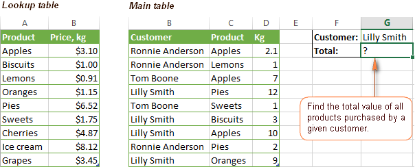
As you remember, you cannot utilize the Excel VLOOKUP function since you have multiple instances of the lookup value (array of data). Instead, you use a combination of SUM and LOOKUP functions like this:
=SUM(LOOKUP($C$2:$C$10,'Lookup table'!$A$2:$A$16,'Lookup table'!$B$2:$B$16)*$D$2:$D$10*($B$2:$B$10=$G$1))
Since this is an array formula, remember to press Ctrl + Shift + Enter to complete it.
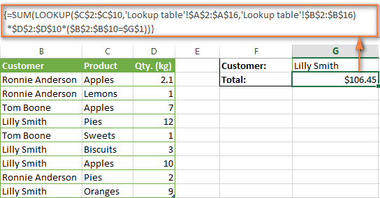
And now, let's analyses the formula's ingredients so that you understand how each of the functions works and can to tweak it for your own data.
We'll put aside the SUM function for a while, because its purpose is obvious, and focus on the 3 components that are multiplied:
LOOKUP($C$2:$C$10,'Lookup table'!$A$2:$A$16,'Lookup table'!$B$2:$B$16)This LOOKUP function looks up the goods listed in column C in the main table, and returns the corresponding price from column B in the lookup table.
$D$2:$D$10This component returns quantity of each product purchased by each customer, which is listed in column D in the main table. Multiplied by the price, which is returned by the LOOKUP function above, it gives you the cost of each purchased product.
$B$2:$B$10=$G$1This formula compares the customers' names in column B with the name in cell G1. If a match is found, it returns "1", otherwise "0". You use it simply to "cut off" customers' names other than the name in cell G1, since all of us know that any number multiplied by zero is zero.
Because our formula is an array formula it iterates the process described above for each value in the lookup array. And finally, the SUM function sums the products of all multiplications. Nothing difficult at all, it is?
Note. For the LOOKUP formula to work correctly you need to sort the lookup column in your Lookup table in ascending order (from A to Z). If sorting is not acceptable on your data, check out an awesome SUM / TRANSPOSE formula suggested by Leo.
Download this LOOKUP and SUM sample
VLOOKUP and SUMIF - look up & sum values with criteria
Excel's SUMIF function is similar to SUM we've just discussed in the way that it also sums values. The difference is that the SUMIF function sums only those values that meet the criteria you specify. For example, the simplest SUMIF formula =SUMIF(A2:A10,">10") adds the values in cells A2 to A10 that are larger than 10.
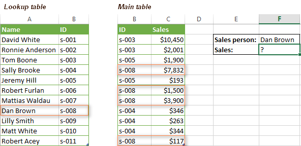
This is very easy, right? And now let's consider a bit more complex scenario. Suppose you have a table that lists the sales persons' names and ID numbers (Lookup_table). You have another table that contains the same IDs and associated sales figures (Main_table). Your task is to find the total of sales made by a given person by their ID. At that, there are 2 complicating factors:
- The mail table contains multiple entries for the same ID in a random order.
- You cannot add the "Sales person names" column to the main table.
And now, let's make a formula that, firstly, finds all sales made by a given person, and secondly, sums the found values.
Before we start on the formula, let me remind you the syntax of the SUMIF function:
range- this parameter is self-explanatory, simply a range of cells that you want to evaluate by the specified criteria.criteria- the condition that tells the formula what values to sum. It can be supplied in the form of a number, cell reference, expression, or another Excel function.sum_range- this parameter is optional, but very important to us. It defines the range where the corresponding cells' values shall be added. If omitted, Excel sums the values of cells that are specified in the range argument (1st parameter).
Keeping the above info in mind, let's define the 3 parameters for our SUMIF function. As you remember, we want to sum all the sales made by a given person whose name is entered in cell F2 in the main table (please see the image above).
- Range - since we are searching by sales person ID, the range parameter for our SUMIF function is column B in the main table. So, you can enter the range B:B, or if you convert you data to a table, you can use the column's name instead:
Main_table[ID] - Criteria - because we have sales persons' names in another table (lookup table), we have to use the VLOOKUP formula to find the ID corresponding to a given person. The person's name is written in cell F2 in the main table, so we look it up using this formula:
VLOOKUP($F$2,Lookup_table,2,FALSE)Of course, you could enter the name in the lookup criteria of your VLOOKUP function, but using an absolute cell reference is a better approach because this creates a universal formula that works for any name input in a given cell.
- Sum range - this is the easiest part. Since our sales numbers are in column C named "Sales", we simply put
Main_table[Sales].Now, all you need is to assemble the formula's parts and your SUMIF + VLOOKUP formula is ready:
=SUMIF(Main_table[ID], VLOOKUP($F$2, Lookup_table, 2, FALSE), Main_table[Sales])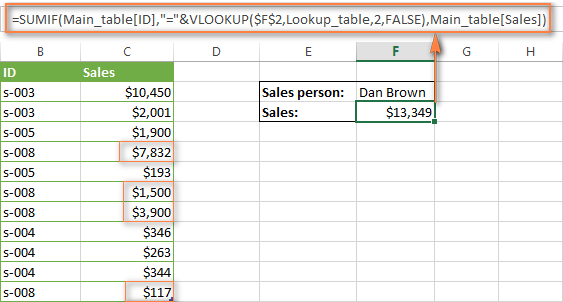
Download this VLOOKUP and SUMIF sample
Formula-free way to do vlookup in Excel
Finally, let me introduce you to the tool that can look up, match and merge your tables without any functions or formulas. The Merge Tables tool included with our Ultimate Suite for Excel was designed and develop as a time-saving and easy-to-use alternative to Excel's VLOOKUP and LOOKUP functions, and it can be very helpful both to beginners and advanced users.
Instead of figuring out formulas, you simply specify your main and lookup tables, define a common column or columns, and tell the wizard what data you want to fetch.
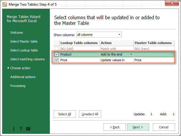
Then you allow the wizard a few seconds to look up, match and deliver you the results. If you think this add-in may prove helpful in your work, you are most welcome to download a trial version by using the below link.
Available downloads
VLOOKUP with SUM and SUMIF - formula examples (.xlsx file)
Ultimate Suite - trial version (.exe file)
 by
by
443 comments
I have the below table
Date Customer PO Number Distributor Name Distributor Country Reseller Name Posid End User Part Number SerialNumber Amount
1/2/2024 22122023_LIC3_SK Exclusive Networks Slovakia s.r.o. Slovakia DATALAN, a.s. FT-131907 DataCentrum elektronizácie územnej samosprávy Slovenska FC-10-F6H0E-108-02-12 0 8727.00
1/2/2024 22122023_LIC3_SK Exclusive Networks Slovakia s.r.o. Slovakia DATALAN, a.s. FT-131907 DataCentrum elektronizácie územnej samosprávy Slovenska FC-10-F6H0E-247-02-12 0 10472.00
1/2/2024 2123080120 DNS a.s. Czech Republic IT AWACS SOLUTION s.r.o. FT-1221865 IT AWACS SOLUTION s.r.o. SP-FG60E-PDC-5 47.00
1/2/2024 K201552 IDEAL SA Greece ALPHA OMEGA ZED LTD FT-1279238 ALPHA OMEGA ZED FS-148F-POE S148FPTF21006236 756.00
1/2/2024 K201552 IDEAL SA Greece ALPHA OMEGA ZED LTD FT-1279238 ALPHA OMEGA ZED FS-148F-POE S148FPTF21006532 756.00
1/2/2024 K202838 IDEAL SA Greece GSLP hellas single member pc FT-1346880 KARANTINOS S.A. FC-10-0060F-950-02-12 249.00
1/2/2024 K202865 IDEAL SA Greece INTTRUST SA FT-122472 INTTRUST S.A. FC-10-F100F-950-02-12 4695.00
1/2/2024 K210478 IDEAL SA Greece ALPHA OMEGA ZED LTD FT-1279238 ALPHA OMEGA ZED FG-100F-BDL-950-12 FG100FTK23004633 2142.00
1/2/2024 K210478 IDEAL SA Greece ALPHA OMEGA ZED LTD FT-1279238 ALPHA OMEGA ZED FG-100F-BDL-950-12 FG100FTK23004714 2142.00
1/2/2024 K210478 IDEAL SA Greece ALPHA OMEGA ZED LTD FT-1279238 ALPHA OMEGA ZED FG-100F-BDL-950-12 FG100FTK23004803 2142.00
1/2/2024 K210478 IDEAL SA Greece ALPHA OMEGA ZED LTD FT-1279238 ALPHA OMEGA ZED FG-100F-BDL-950-12 FG100FTK23006714 2142.00
and need to extract to another sheet the sum of column "Amount" that refers to POSID "FT-1279238"
what is the formula?
Hello Marilena!
To calculate the amount by condition, you can use the SUMIF or SUMIFS function. For example:
=SUMIF(J2:J12,"FT-1279238",Q2:Q12)
You can find detailed instructions on how to reference a formula from one worksheet to another in the correct manner here: Excel reference to another sheet or workbook (external reference).
Hi, I have a daily timesheet which I want to link to Tracker in excel. My formula i used is the following =IFERROR(VLOOKUP (C17:C35,'Anthea (2)'! $B$4: $F$18,5,0)," "). However, due to the fact that a person will do the same task more than once a day but at different times my formula only calculated the first instance the person perform the task and does not sum it.
Hi! To sum by condition, you can use the SUMIFS formula. You can find the examples and detailed instructions here: Excel SUMIFS and SUMIF with multiple criteria.
You can also calculate the sum by conditions using the SUMPRODUCT formula
I hope it’ll be helpful. If something is still unclear, please feel free to ask.
Hi,
Appreciate that if can help recommend the most suitable formula can apply for tlbelow scenario.
Individual name (ColumnA)
Activity name (column B)
Daily numbers in month(from column C -day 1 till end of month 31)
how to get daily sum total for same activity type from multiple individual name?
Hi! If I understand your task correctly, to find the sum of several conditions, you can use the SUMPRODUCT formula.
The formula might look as follows:
=SUMPRODUCT(C2:AG10*(B2:B10="Activity")*((A2:A10="Name1")+(A2:A10="Name2")))
You can find the examples and detailed instructions here: Excel SUMPRODUCT function with multiple criteria.
Hi I tried apply the formula above but shown #value!
Column A2:A5 different name
Column B2:B5 multiple activities eg. Running, dancing..etc
Row C2,D2...etc referring to day 1,2,3..
If to sum up all individuals who attend running activities for day 1. Subsequently sum running numbers for day 2...etc
Next sum all individual who attend dancing activity for day 1. Subsequently repeat same sum for day 2 till month end.
Hi! I wrote this formula based on the description you provided in your original comment. However, if you read the recommended article carefully, you can easily modify the formula for your task. For example, running activities for day 1:
=SUMPRODUCT(C2:C10*(B2:B10="Running"))
Or you can use the SUMIF formula:
=SUMIF(B2:B10,"Running",C2:C10)
To automatically summarize by day number, you can try this formula:
=SUMPRODUCT(C2:AG10*(B2:B10="Running")*(C1:AG1=1))
You can replace the number "1" in the formula with a reference to the cell with the day number.
How to do i use the vlookup function when i have 2 value needed to sum correspondently.
For instance,
Column A (name)
Ester
Ester
John
John
Susan
Column B (Date)
31/08/22
22/08/22
22/08/22
31/08/22
31/08/22
Column C (spending)
$32.00
$148.00
$25.00
$16.00
$36.00
How to write a formula that correspond to Ester for only spending 22/08/22.
Hello Jason!
To find the last match, you can use the XLOOKUP function. Look for the example formulas here: XLOOKUP in reverse order to get last occurrence. The formula might look like this:
=XLOOKUP("Ester",A1:A10,B1:B10,,0,-1)
You can also try the INDEX XMATCH formula. Read more about the XMATCH function here: Excel XMATCH function with formula examples. For example:
=INDEX(B1:B10,XMATCH("Ester",A1:A10,0,-1))
If these functions are not available to you, create an helper column D. In cell D1, use the following formula and drag it down to apply to all cells:
=IF(A1="Ester", COUNTIF($A$1:A1, "Ester"), "")
Use the INDEX and MATCH functions to find the second occurrence of "Ester" and return the corresponding date from Column B.
In a new cell (for example, E1), use the following array formula:
=INDEX(B1:B10,MATCH(MAX(D1:D10),D1:D10,0))
hai,
please help me
I want to know the formula for taking a price list like this, based on the valid date from - valid to,
id(a) valid from(b) valid to(c) price(d)
8481 1/25/2024 5/31/2024 104,727
8481 6/3/2024 10/16/2024 109,968
8481 10/17/2024 121,730
2/25/2024 8481
6/30/2024 8481
10/23/2024 8481
Hi! If I understand your task correctly, the following tutorial should help: Excel INDEX MATCH with multiple criteria - formula examples. For example:
=INDEX(D1:D10,MATCH(1,(A1:A10=H1)*(B1:B10<=G1)*(C1:C10>=G1),0))
Please ensure that all dates in columns B and C are entered.
H1 & G1 what colomns?
Read carefully how the INDEX MATCH function works with multiple criteria.
H1 - date 2/25/2024, G1 - ID 8481
I need a formula that will select specific numbers from cells in column A that add up to a number that I put into cell C2. I would like excel to return an X in column b next to the selected cells in column A
Hello Lisa!
If I understand your task correctly, the following tutorial should help: Find all combinations of numbers that equal a given sum in Excel.
You can also use the Solver tool. Read the detailed instructions here: Excel Solver tutorial with step-by-step examples.
How to use SUMIF and VLOOKUP in multiple excel files ?
Hi! You cannot use VLOOKUP with SUMIF in multiple Excel files. You can merge these files and then do calculation with VLOOKUP. Maybe this article will be helpful: How to merge Excel files into one.
how can i sum the item in each value?
Clarify your specific problem or provide additional details to highlight exactly what you need.
How to Find Over all Total Value in Single Name - Vlookup
Hi! Have you tried any of the methods described in this blog post? If they don't work for you, please describe your problem in detail and I'll have a look at a possible solution.
Hi! I am gathering scores from about 100 football matches. There are 5 columns. Date, Home, Score 1, Away, Score 2. Some teams played multiple matches and I want to get the total accumulated scores of all teams that played.
Hi! Since your columns do not include the team name, your question is not entirely clear. On the basis of your information, I think you can calculate the sum scores by condition with the help of the SUMIFS function. If this does not help, explain the problem in detail.
There is a team name, on the 2nd and 3rd column.
=SUM(VLOOKUP(H3,$B$3:$E$14, 2, FALSE))
I actually used this formula but for some reason, it only shows the score on the first game and not the accumulated scores of different matches.
Hi! The VLOOKUP function will only return the first result that it finds. So use the SUMIFS function from my earlier recommendation.
For example:
=SUMIF(B3:B10,H3,C3:C10)
You can also use this tutorial: Excel SUMPRODUCT function with formula examples. The formula might look something like the following:
=SUMPRODUCT((B3:B10=H3)*C3:C10)
Actually .i have a concern that telecom company there is so many account number,
Account Number Amount
1.324567777 300
1.324567777 300
1.345677890 -40
1.345677890 20 I want to want the account duplicate and same time i want to get the total amount in one account in one column by using formulae ,can you please me regarding this concern using sumif
Like this format
Account Number Amount
1.324567777 600
1.324567777 0
1.345677890 20
1.345677890 0
Thankyou
Chithra
Hi! You can learn more about sum by condition in this article: How to use SUMIF function in Excel with formula examples. For example:
=SUMIF(A1:A100,A1,B1:B100)
To get the amount for each Account Number, you can also use a Pivot Table.
Thanks for the info,
can you help me, i have a question. for a big data how do i make a dynamic refereance for {2,3,4,5,6,7,8,9,10,11,12,13}.
created a manual serie. {8;9;10;11;12;13;14;15;16;17;18;19;20;21;22;23;24;25;26;27;28;29;30;31;32;33;34;35;36;37;38;39;40;41;42;43;44;45;46;47;48;49;50;51;52;53;54;55;56;57;58;59}
but it is so hard to keep the formula updated all the weeks
ıt should start with H (8th) colulmn and finish at the end of the year.
Hi! What do you want to calculate exactly? What formula you used? Your question is not entirely clear, please specify.
Hello, I have 3 columns
Name ID Amounts I want to get sum of amounts in a cell where I write Names , some rows might be exactly same in the worksheet
AA 22 200
AA 22 200
AA 33 100
BB 11 300
so when I type AA in a cell, I want to get 100+200=300 value not 200+200+100=500 , so I want excel to sum only different amounts of the same name
I have cell where names are written for example AA and I want to put sum of amounts next to The Name cell
P.S
My worksheet needs to have duplicate rows, I can't delete them
And I don't have UNIQUE function on my excel
Hi! In your version of Excel, I recommend copying the data to a separate sheet and removing duplicate rows. You can use the Duplicate Remover tool to remove duplicate rows. You can then use the COUNTIFS function to calculate count by condition.
You can also find useful information in this article: How to remove duplicates in Excel (duplicate rows, values and partial matches).
and I want SUM of amounts not Count
You remove duplicates from the copy of your data. To find the sum by condition, use the SUMIFS function.
Duplicate remover tool is available as a part of our Ultimate Suite for Excel that you can install in a trial mode and check how it works for free.
yes, but I need to have duplicates
I have a delivery record for 10 years for more than 1000 items.
I need to know each item last delivery year. What is the formula that I can use to identify each item last delivery year?
Hi! You can get the records for the desired year with the FILTER function. Then use the UNIQUE function to get a list of items without duplicates. You can find the examples and detailed instructions here: Get a list of unique values based on criteria.
im trying to apply this to my sheet, but am getting stuck, i have unique ids instead of names, the ids are in 2 seperate tables, i need to subtract table 1 from table 2 based on id number..
could this be done using this method or am i looking for another way?
table 1
id, games lost, total value
1 5 100
2 12 1500
3 3 1200
table 2
id, games won, total value
1 7 1100
2 1 2500
3 9 800
table 3
id, total games played, total value
1 7
2 13
3 12
table 3 will be the total profit/ loss
if this make sense
Hi! If I understand your task correctly, you are trying to use the SUMIFS function to sum values by condition:
=SUMIFS(Sheet2!C1:C10,Sheet2!A1:A10,Sheet3!A1) - SUMIFS(Sheet1!C1:C10,Sheet1!A1:A10,Sheet3!A1)
For more information, please visit: How to use Excel SUMIFS and SUMIF with multiple criteria.
Hello,
I have an excel sheet with client names in Column A and the corresponding revenue for the last 24 months. I want to organise the the customers based on the highest revenue for each month. How can i do this in excel.
Hi! Based on your description, it is hard to completely understand your task. If you want to sort customers, use the SORT function as described in this manual: Excel SORT function - auto sort data using formula. You can also use these guidelines: How to alphabetize in Excel: sort columns and rows A-Z or Z-A. If this does not help, explain the problem in detail.
Hi Alex,
I have a list of projects (column a) and man hours (column b). I want to total the man hours for the projects that contain “PI17” anywhere in their project name.
What would you suggest?
Thank you
Hi! Identify the cells that contain the text you want. For more information, please read: How to find substring in Excel. Then use the SUMPRODUCT function to sum the numbers corresponding to the selected cells. For example:
=SUMPRODUCT(--(ISNUMBER(SEARCH("PI17",A1:A10))),B1:B10)
Thanks for your help. That worked great!
I have an issue, I have a data validation list (Product Name) in sheet A, in sheet B i have the same data but in a simple list but with a second value in column B (Commission Rate that applies to Product) . I want to return the value in column B based on what I select in drop down on Sheet A
Hi! You can search for the Product Name, that is selected in the drop-down list, in the list on worksheet B. To extract the corresponding Commission Rate value from column B on worksheet B, use the VLOOKUP formula as described in this manual: How to Vlookup from another sheet in Excel. I hope I answered your question. If something is still unclear, please feel free to ask.
01-Aug-23 Ahmed RK 10000
01-Aug-23 Akash RK 20000
01-Aug-23 Ahmed KH 30000
01-Aug-23 Akash KH 40000
02-Aug-23 Ahmed RK 50000
02-Aug-23 Akash RK 60000
02-Aug-23 Ahmed KH 70000
02-Aug-23 Akash KH 80000
Dear Friend
i need google sheets SUM formula of
01-Aug-23 RK 30000 (SUM : 10000+20000)
01-Aug-23 KH 70000
02-Aug-23 RK 110000
Hi.
Although I can use the VLOOK function OK, I do have a problem I cant resolve.
So, VLOOKUP returns a number (In this case an amount of money)
I want to multiply this with another column value that is a qunatity to get a total
All I get back is #NAME?
Thanks - in advance.
Andrew
Hi. I can't guess which formula you are using. However, you are incorrectly writing the name of the Excel function. This is indicated by the error #NAME?
SIGH ... ignore this question. Blame it on a senor moment...!
Hi
please help me
I have two columns which are headers Month & Revenue
line January, February, March etc and the second col 1000, 2000, 3000
I need a formula to add upto the month i.e. when i need upto february sum of above month January and February (1000+2000=3000)
and similarly march shoud results 1000+2000+3000
thanks in advance
Hello!
If I understand your task correctly, you can also find useful information in this article: How to do a running total in Excel (Cumulative Sum formula). If this does not help, explain the problem in detail.