A while ago we started to explore the capabilities of Excel Data Validation and learned how to create a simple drop-down list in Excel based on a comma-separated list, range of cells or a named range.
Today, we are going to investigate this feature in-depth and learn how to create cascading drop down lists that display choices depending on the value selected in first dropdown. To put it differently, we will make an Excel data validation list based on the value of another list.
How to create multiple dependent dropdown in Excel
Making a multi-level dependent drop-down lists in Excel is easy. All you need is a few named ranges and the INDIRECT formula. This method works with all versions of Excel 365 - 2010 and earlier.
1. Type the entries for the drop-down lists
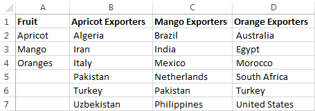
First off, type the entries you want to appear in the drop-down lists, each list in a separate column. For example, I'm creating a cascading dropdown of fruit exporters and column A of my source sheet (Fruit) includes the items of the first dropdown and 3 other columns list the items for the dependent dropdowns.
2. Create named ranges
Now you need to create names for your main list and for each of the dependent lists. You can do this either by adding a new name in the Name Manager window (Formulas tab > Name Manager > New) or typing the name directly in the Name Box.
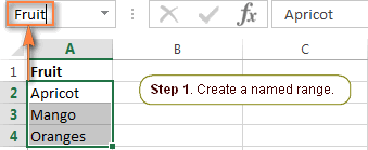
Note. Please pay attention that if your first row is sort of column header like you see in the screenshot above, you shall not include it in the named range.
For the detailed step-by-step instructions please see How to define a name in Excel.
Things to remember:
- The items to appear in the first drop-down list must be one-word entries, e.g. Apricot, Mango, Oranges. If you have items consisting of two, three or more words, please see How to create a cascading dropdown with multi-word entries.
- The names of the dependent lists must be exactly the same as the matching entry in main list. For example, the dependent list to be displayed when "Mango" is selected from the first drop-down list should be named Mango.
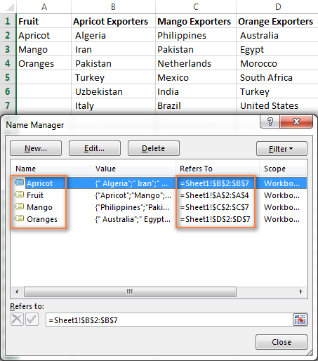
When done, you may want to press Ctrl+F3 to open the Name Manager window and check if all of the lists have correct names and references.
3. Make the first (main) drop-down list
- In the same or in another spreadsheet, select a cell or several cells in which you want your primary drop-down list to appear.
- Go to the Data tab, click Data Validation and set up a drop-down list based on a named range in the usual way by selecting List under Allow and entering the range name in the Source box.
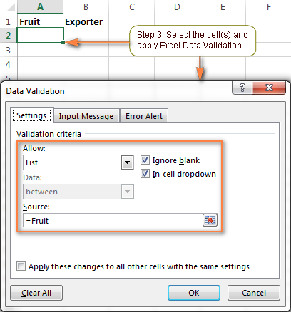
For the detailed steps, please see Making a drop down list based on a named range.
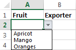
As the result, you will have a drop-down menu in your worksheet similar to this:
4. Create the dependent drop-down list
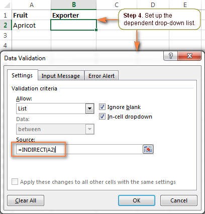
Select a cell(s) for your dependent drop-down menu and apply Excel Data Validation again as described in the previous step. But this time, instead of the range's name, you enter the following formula in the Source field:
=INDIRECT(A2)
Where A2 is the cell with your first (primary) drop-down list.
If cell A2 is currently empty, you will get the error message "The Source currently evaluates to an error. Do you want to continue?"
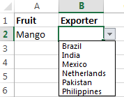
Safely click Yes, and as soon as you select an item from the first drop-down menu, you will see the entries corresponding to it in the second, dependent, drop-down list.
5. Add a third dependent drop-down list (optional)
If needed, you could add a 3rd cascading drop-down list that depends either on the selection in the 2nd drop-down menu or on the selections in the first two dropdowns.
Set up 3rd dropdown that depends on 2nd list
You can make the drop-down list of this type in the same fashion as we've just made a second dependent drop-down menu. Just remember the 2 important things discussed above, which are essential for the correct work of your cascading drop-down lists.
For instance, if you want to display a list of regions in column C depending on which country is selected in column B, you create a list of regions for each country and name it after the country's name, exactly as the country appears in second dropdown lists. For instance, a list of Indian regions should be named "India", a list of Chines regions - "China", and so on.
After that, you select a cell for the 3rd dropdown (C2 in our case) and apply Excel Data Validation with the following formula (B2 is the cell with the second drop-down menu that contains a list of countries):
=INDIRECT(B2)
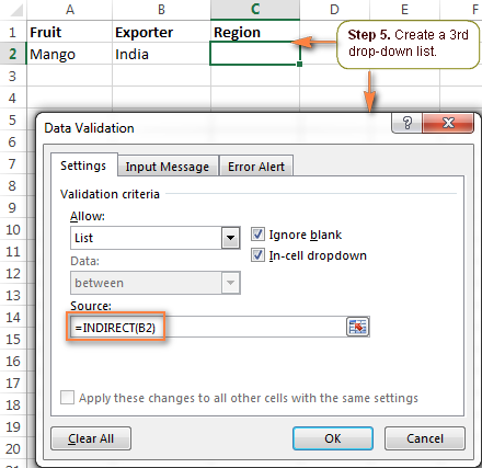
Now, each time you select India under the list of countries in column B, you will have the following choices in the third drop-down:
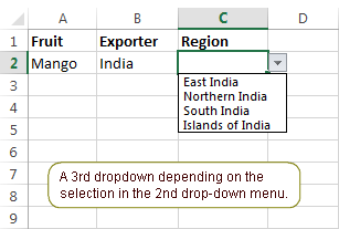
Note. The displayed list of regions is unique for each country but it does not depend on the selection in the first drop-down list.
Create a third dropdown dependent on the first two lists
If you need to create a cascading drop down menu that depends on the selections both in the first and second drop-down lists, then proceed in this way:
- Create additional sets of named ranges, and name them for the word combinations in your first two dropdowns. For example, you have Mango, Oranges, etc. in the 1st list and India, Brazil, etc. in the 2nd. Then you create named ranges MangoIndia, MangoBrazil, OrangesIndia, OrangesBrazil, etc. These names should not contain underscores or any other additional characters.
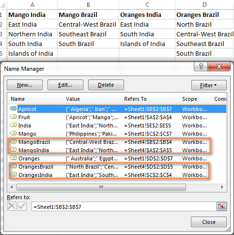
- Apply Excel Data Validation with the INDIRECT SUBSTITUTE formula that concatenates the names of the entries in the first two columns, and removes the spaces from the names. For example, in cell C2, the data validation formula would be:
=INDIRECT(SUBSTITUTE(A2&B2," ",""))Where A2 and B2 contain the first and second dropdowns, respectively.
As the result, your 3rd drop-down list will display the regions corresponding to the Fruit and Country selected in the first 2 drop-down lists.
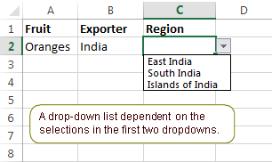
This is the easiest way to create cascading drop-down boxes in Excel. However, this method has a number of limitations.
Limitations of this approach:
- The items in your primary drop-down list must be one-word entries. See how to create cascading drop-down lists with multi-word entries.
- This method won't work if the entries in your main drop-down list contain characters not allowed in range names, such as the hyphen (-), ampersand (&), etc. The solution is to create a dynamic cascading dropdown that does not have this restriction.
- Drop-down menus created in this way are not updated automatically i.e. you will have to change the named ranges' references every time you add or remove items in the source lists. To get over this limitation, try making a dynamic cascading drop down list.
Create cascading drop-down lists with multi-word entries
The INDIRECT formulas that we used in the example above can handle one-word items only. For example, the formula =INDIRECT(A2) indirectly references cell A2 and displays the named range exactly with the same name as is in the referenced cell. However, spaces are not allowed in Excel names, which is why this formula won't work with multi-word names.
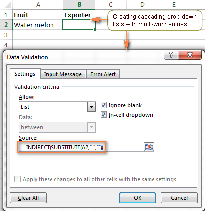
The solution is to use the INDIRECT function in combination with SUBSTITUTE like we did when creating a 3rd dropdown.
Suppose you have Water melon among the products. In this case, you name a list of water melon exporters with one word without spaces - Watermelon.
Then, for the second dropdown, apply Excel Data Validation with the following formula that removes the spaces from the name in cell A2:
=INDIRECT(SUBSTITUTE(A2," ",""))
How to prevent changes in the primary drop down list
Imagine the following scenario. Your user has made the selections in all of the drop-down lists, then they changed their mind, went back to the first list, and chose another item. As the result, the 1st and 2nd selections are mismatched. To prevent this from happening, you may want to block any changes in the first drop-down list as soon as a selection is made in the second list.
To do this, when creating the first dropdown, use a special formula that will check whether any entry is selected in the second drop down menu:
=IF(B2="", Fruit, INDIRECT("FakeList"))
Where B2 contains the second dropdown, "Fruit" is the name of the list that appears in the first drop-down menu, and "FakeList" is any fake name that does not exist.
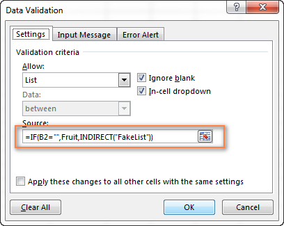
Now, if any item is selected in the 2nd drop-down list, no choices will be available when the user clicks on the arrow next to the first list.
Creating dynamic cascading drop-down lists in Excel
The main advantage of a dynamic Excel dependent drop-down list is that you are free to edit the source lists and your drop-down boxes will get updated on the fly. Of course, creating dynamic dropdowns requires a bit more time and more complex formulas, but I believe this is a worthy investment because once set up, such drop-down menus are real pleasure to work with.
As with almost anything in Excel, you can achieve the same result in several ways. In particular, you can create a dynamic dropdown using a combination of OFFSET, INDIRECT and COUNTA functions or a more resilient INDEX MATCH formula. The latter is my preferred way because it provides numerous advantages, the most essential of which are:
- You have to create 3 named ranges only, no matter how many items there are in the main and dependent lists.
- Your lists may contain multi-word items and any special chars.
- The number of entries can vary in each column.
- The entries' sort order does not matter.
- Finally, it's very easy to maintain and modify the source lists.
Okay, enough theory, let's get to practice.
1. Organize your source data in a table
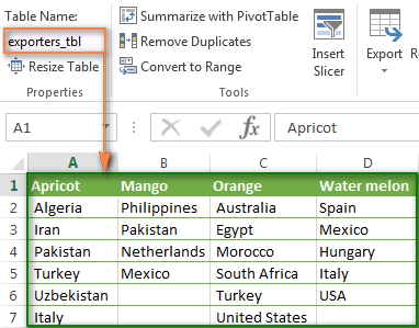
As usual, the first thing for you to do is to write down all the choices for your drop-down lists in a worksheet. This time, you will have store the source data in an Excel table. For this, once you have entered the data, select all of the entries and press Ctrl + T or click Insert tab > Table. Then type a name of your table in the Table Name box.
The most convenient and visual approach is to store the items for the first drop-down as table headers, and the items for the dependent dropdown as table data. The screenshot below illustrates the structure of my table, named exporters_tbl - the fruit names are table headers and a list of exporting countries is added under the corresponding fruit name.
2. Create Excel names
Now that your source data is ready, it's time to set up named references that will dynamically retrieve the correct list from your table.
2.1. Add a name for the table's header row (main dropdown)
To create a new name that references the table header, select it and then either click Formulas > Name Manager > New or press Ctrl + F3.
Microsoft Excel will use the built-in table reference system to create the name of the table_name[#Headers] pattern.
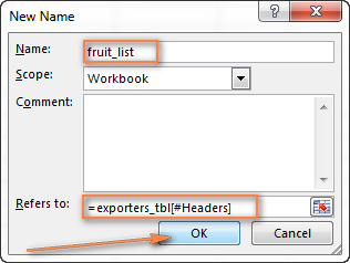
Give it some meaningful and easy to remember name, e.g. fruit_list, and click OK.
2.2. Create a name for the cell containing the first drop-down list
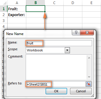
I know that you don't have any dropdown yet :) But you have to choose the cell to host your first dropdown and create a name for that cell now because you will need to include this name in the third name's reference.
For example, my first drop-down box is reside in cell B1 on Sheet 2, so I create a name for it, something simple and self-explanatory like fruit:
Tip. Use appropriate cell references to copy drop-down lists across the worksheet.
Please be sure to read the following few paragraphs carefully because this a very useful tip you that don't want to miss. Thanks a lot to Karen for posting it!
If you plan to copy your drop-down lists to other cells, then use mixed cell references when creating the name for the cell(s) with your first drop-down list.
For the drop-downs to copy correctly to other columns (i.e. to the right), use relative column (without the $ sign) and absolute row (with $) references like = Sheet2!B$1.
As the result, B1's dependent drop down list will appear in cell B2; C1's dependent drop-down will display in C2, and so on.
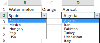
And if you plan to copy the dropdowns to other rows (i.e. down the column), then use absolute column (with $) and relative row (without $) coordinates like = Sheet2!$B1.
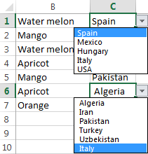
To copy a drop-down cell in any direction, use a relative reference (without the $ sign) like = Sheet2!B1.
2.3. Create a name to retrieve the dependent menu's entries
Instead of setting up unique names for each of the dependent lists like we did in the previous example, we are going to create one named formula that is not assigned to any particular cell or a range of cells. It will retrieve the correct list of entries for the second dropdown depending on which selection is made in the first drop-down list. The main benefit of using this formula is that you won't have to create new names as you add new entries to the first drop-down list - one named formula covers them all.
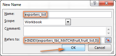
You create a new Excel name with this formula:
=INDEX(exporters_tbl,,MATCH(fruit,fruit_list,0))
Where:
exporters_tbl- the name of the table (created in step 1);fruit- the name of the cell containing the first drop-down list (created in step 2.2);fruit_list- the name referencing the table's header row (created in step 2.1).
I gave it a name exporters_list, as you see in the screenshot below.
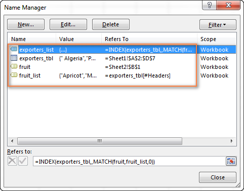
Well, you have already done the major part of the work! Before getting to the final step, it may be a good idea to open the Name Manager (Ctrl + F3) and verify the names and references:
3. Set up Excel Data Validation
This is actually the easiest part. With the two named formulas in place, you set up Data Validation in the usual way (Data tab > Data validation).
- For the first drop-down list, in the Source box, enter =fruit_list (the name created in step 2.1).
- For the dependent drop-down list, enter =exporters_list (the name created in step 2.3).
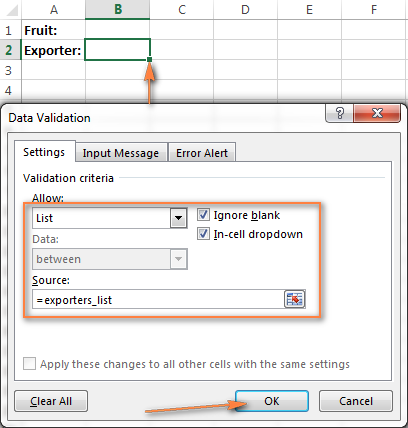
Done! Your dynamic cascading drop-down menu is accomplished and will update automatically reflecting the changes you've made to the source table.
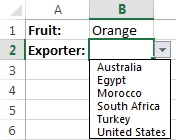
This dynamic Excel dropdown, perfect in all other respects, has one shortcoming - if the columns of your source table contain a different number of items, the blank rows will appear in your menu like this:
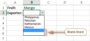
Exclude blank rows from the dynamic cascading dropdown
If you want to clean any blank lines in your drop-down boxes, you will have to take a step further and improve the INDEX / MATCH formula used to create the dependent dynamic drop-down list.
The idea is to use 2 INDEX functions, where the first gets the upper-left cell and the second returns the lower-right cell of the range, or the OFFSET function with nested INDEX and COUNTA. The detailed steps follow below:
1. Create two additional names
Not to make the formula too bulky, create a couple of helper names with the following simple formulas first:
- A name called col_num to reference the selected column number:
=MATCH(fruit,fruit_list,0) - A name called entire_col to reference the selected column (not the column's number, but the entire column):
=INDEX(exporters_tbl,,col_num)
In the above formulas, exporters_tbl is your source table's name, fruit is the name of the cell containing the first dropdown, and fruit_list is the name referencing the table's header row.
2. Create the named reference for the dependent dropdown
Next, utilize either of the below formulas to create a new name (let's call it exporters_list2) to be used with the dependent drop-down list:
=INDEX(exporters_tbl,1,col_num) : INDEX(exporters_tbl, COUNTA(entire_col), col_num)
=OFFSET(INDEX(exporters_tbl,1,col_num),0,0,COUNTA(entire_col))
3. Apply Data Validation
Finally, select the cell containing the dependent dropdown and apply Data Validation by entering = exporters_list2 (the name created in the previous step)in the Source box.
The screenshot below shows the resulting dynamic drop-down menu in Excel where all blank lines are gone!
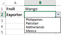
Note. When working with dynamic cascading drop down lists created with the above formulas, nothing prevents the user from changing the value in the first dropdown after making the selection in the second menu, as a result, the choices in the primary and secondary dropdowns may mismatch. You can block changes in the first box after a selection is made in the second one by using either VBA or complex formulas suggested in this tutorial.
This is how you create an Excel data validation list based on the values of another list. Please feel free to download our sample workbooks to see the cascading drop-down lists in action. Thank you for reading!
Practice workbook for download
Cascading Dropdown Sample 1- easy version
Cascading Dropdown Sample 2 - advanced version without blanks
 by
by
151 comments
Thankyou for sharing knowledge. I want to make a excel sheet that have brand, item type, item name, price, etc. Requirement is when I select the brand and the Item Type, next cell I could able to select a item name only matches to both brand and item type. Ex: I select ABB as brand and MCCB as Item type. Under the Item name I want to select ABB MCCB that I want from a drop down. Then next row I select ABB as brand and ACB as item type. Next cell of same row it should be show all ABB ACBs to select the one I wanted. Problem is excel don't support to use formula as data validation source. Any options??
Hi! I think you can find a solution to your problem in the article above. I also recommend paying attention to these recommendations: Create a dynamic dependent drop down list in Excel an easy way.
Does this work on Excel online? In the "Source" field, when I input =INDIRECT($D$2) it works, but when I input =INDIRECT(D2) (without the $) it gives me the error message "This entry leads to an error. Try entering different values to continue".
Hi! Formula INDIRECT($D$2) works because it always points to one fixed cell (D2) which contains your list name or reference.
Formula INDIRECT(D2) fails in that dialog because Excel Online is stricter — it does not treat relative references as valid inside the Source box.
It expects either:
absolute reference ($D$2),
or a hard-coded string (like =Apples),
or a named range.
In Excel Online, the validation UI rejects it as ambiguous, so you get error message.
If you need relative behavior per row, define a named formula that uses =INDIRECT(D2) and then point Data Validation to the named formula. This gets around the Source field limitation. Read more: How to make a named formula.
I am not getting step 4 in "Making a dependent (cascading) drop down list in Excel" working. When I enter the formula as defined in the steps it give me the list of options from column 1 (named range) again. I am not understanding how it would know that the value in the referenced field (A2) is referring to a named range.
Hi! Verify that you have created the named ranges correctly as described in Step 2. In Step 4, you select the name of one of these named ranges using the INDIRECT function. Read more: INDIRECT with named ranges.
thank you for making this kind of tutorial :) it's so helpful
Hi, thank you for the tutorial.
Is there a way to define the source of the dependent drop down list as its corresponding cell in a table column?
What I mean is that I have a table named "Prog_list" with a lot of rows (which makes your approach of creating a name for each cell impractical), in one of the table's column (named "Category") I set up the first drop down list. What I want to do is to have the cell in "Category" to be the source of the dependent drop down list to be found in a separate column named "Sub_Category". I tried the formula "=INDIRECT(Prog_List[@[Category]])" but I got an error.
Hi! INDIRECT(Prog_List[@[Category]]) doesn’t work because INDIRECT requires text reference to named range or defined address, and structured table references don’t play well with it.
I recommend reading this guide: Excel INDIRECT function - basic uses and formula examples.
You can define the source for the dependent drop-down by creating named range with dynamic formula. For example:
=INDEX(Sub_Category_List,MATCH([@Category],Category_List,0))
where:
Sub_Category_List - refers to the column containing possible subcategories.
Category_List - refers to the column containing main categories.
If you’re using Excel 365 or Excel 2019 with dynamic array functions, try this formula:
=FILTER(Sub_Category_List, Category_List=[@Category])
Read more: Excel FILTER function - dynamic filtering with formulas.
This approach dynamically pulls relevant subcategories based on the selected main category.
Then, set this named range as the source for the dependent drop-down list.
Hello,
I am trying to create multilevel drop down in one cell. I have seen it on a couple of different sites and would like to incorporate into a checklist. What I mean is, when you click on the drop down and hover on "Yes" then another dropdown will automatically show other options to go along with the "Yes" response "Yes, this item has been completed..." or "Yes, this doesn't need to be done..". Or "No, this is not needed", etc.?
Hello Heather!
This is not possible with the standard Excel options. This can be done using a VBA macro.
Hey, Great Tutorial. But Is there a way to have two Dependent Drop Down Lists On only one drop down list?
Hello Brian!
You can create a second dependent drop-down list in another cell in the same way you created the first dependent drop-down list.
Hi Alexander,
I've got a drop-down list already and want to link simplified charts to each name in that drop-down list to the nearby cell.
So that when I chose Steel, to have one graph in that cell.
But when I chose Aluminum - to have another graph in that same cell.
Can you Email me with the solution, please?
I'm sure it's something simple but I simply cannot find it.
Kind regards
p.s. I guess I have to have another sheet where to link each Metal to specific values (in order to have a simple graphic), but don't know how to link the drop-down list to that "graph" cell (on the main page)
Hello Petar!
You can create a drop-down list in the cell you are using to create the diagram. Then the graph will change when you use the drop-down list.
I recommend reading this guide: Customize a chart created from several sheets.
Great tutorial, I'm working on a two column drop down and I've got it all set up so it works but I want to make it more efficient. Is there a way to get the second column to automatically populate if the selection in the first dropdown would only allow a single option in the second column dropdown ?
Thanks in advance!
Hi! Automatic filling of the drop-down list is not supported by Excel. But you can do it using VBA.
Many thanks, I have used your example to set up a dependent drop down. I want to adapt this example across 25 different columns. The only change will be the cell for 'fruit', which will be B6, C6, D6 etc. Could you advise on the best way to do this without having to repeat each exporters list multiple times?
Hi! Unfortunately, I don't really understand what it is you are trying to do. The macros suggested in this article will work with any drop-down lists. You may be able to use one of the methods described in this article to create the dependent dropdown list that you need: Create a dynamic dependent drop down list in Excel an easy way.
Loved this tutorial. Very helpful and thank you for posting but one question. How can I put this IF function....=IF(B2="", Fruit, INDIRECT("FakeList"))...to prevent changes to the primary drop down in the Data Validation Source Field for the first drop down list when I already the Named Range function in this field?
Hi! I'm afraid I don't really understand your question and your formula. If you change the data source for the drop-down list in any way, drop-down list will change as well.
Maybe this article will be helpful: How to lock and unlock cells in Excel.
Hey, I was able to get the two columns to work for the dynamic drop-down list, but I am unable to repeat this process in the next row even with special paste "Validation".
Using your method of dynamic drop-down listing...is there a way I can quickly repeat the same drop-down list but in the next row?
Hi! I don't know how you created your dynamic dropdown list and what formulas you used to create it. But I recommend to use absolute cell references in these formulas, which will not change when copying the dropdown list.
I hope it’ll be helpful. If this is not what you wanted, please describe the problem in more detail.
Hi.
I've been looking for a method of creating dependent drop downs using "INDIRECT()" which sorts and removes blanks.
I thought "UNIQUE()" and "SORT()" would work but the setting for "Data Validation" dialog box doesn't seem to like it.
Thoughts?
Thanks in advance for your consideration.
Hi! If the recommendations in this article don't work for you, try these: Create a dynamic dependent drop down list in Excel an easy way.
Hi,
I notice from the example above during the preparation the columns for dependent dropdown are filled manually.
Is there a way to make it filled automatically? Because I have a really long data as the main drop down, and all the data are filtered from another table.
Hi! If I understand your task correctly, this article may be helpful: How to create drop down list in Excel: dynamic, editable, searchable.
Hi, I have a table listing foods in a column and each food has a row of nutritional values associated with the food listed in that row. I am trying to select several foods that are eaten for a meal and have the corresponding row of data populated on a sheet where all of the selected values in each column are summed up for daily nutritional totals for the day. Any hint on how to select from a list of foods and capture the nutritional data for summing?
Thanks!
Bill
Hi! You can choose each product in a separate cell using the drop-down list. In the next column, get the nutritional value data using VLOOKUP. I recommend reading this guide: Excel VLOOKUP function tutorial with formula examples.
This was very helpful, thank you for that.
Is it possible to have a primary table with multiple dependent tables?
For example, I have a table with 30 Organizations. Each of those organizations have a unique list of Areas, Departments, and accounts.
Hi! In each dependent drop down list, you can select the same main drop down list if you need to. But when you change the main drop down list, you must change the 30 other dependent drop down lists.
Hi I have two workbooks - my source workbook is named "Backend Data" and my destination workbook is named as "Work Instruction".
In my source workbook there is a sheet named R50 with column D named Products and has different Products in this column. I want use this column D as a reference to get values in a single cell in my destination workbook. this single cell should then act as a dropdown list with the contents of the column D from my source workbook. I have tried everything such as named range, index, vlookup but still stuck please help
Hi! If I understand your task correctly, the following tutorial should help: Make drop-down menu from a range of cells. I hope it’ll be helpful.
I get the first drop down to work, but the second one has nothing. I tried it with my data and nothing. Then I created a new document and used the data in this tutorial and get nothing. Ideas?
Hi! Try using the sample file linked at the end of this article. Or carefully follow all the recommendations described above. If you do everything correctly, the multiple selection macro will work.
I am preparing students report and I need a formula that will lookup values of a specific student based on the selected term.
I used vlookup for only one term and it is working but how do I fetch their marks based on selected terms?
Hi! For the VLOOKUP formula, each term must be specified in a separate cell. To give more precise advice, please describe the problem in more detail.
Hi,
Is there a way to sort the data in the "Source Table"?
When I sort the data in the 1st column, the other columns are also reordered.
Your example has short lists of data that are easy to sort by hand, but for longer lists (and less experienced Excel users) it becomes more difficult to do.
Hi! Before creating named ranges and converting a range of values to a Source table, sort the values in each data column. This will work if no new data is added.