This tutorial explains the difference between the SUMIF and SUMIFS functions in terms of their syntax and usage, and provides a number of formula examples to sum values with multiple AND / OR criteria in Excel 365, 2021, 2019, 2016, 2013, 2010, and lower.
As everyone knows, Microsoft Excel provides an array of functions to perform various calculations with data. A few articles ago, we explored COUNTIF and COUNTIFS, which are designed for counting cells based on a single condition and several conditions, respectively. Last week we covered Excel SUMIF that adds values meeting the specified criteria. Now it's time to go over the plural version of SUMIF - Excel SUMIFS that allows summing values by multiple criteria.
Those who are familiar with the SUMIF function might think that converting it to SUMIFS takes just an extra "S" and a few additional criteria. This would seem quite logical… but "logical" it's not always the case when dealing with Microsoft : )
Excel SUMIF function - syntax & usage
The SUMIF function is used to conditionally sum values based on a single criteria. We discussed the SUMIF syntax in detail in the previous article, and here's just a quick refresher.
- range - the range of cells to be evaluated by your criteria, required.
- criteria - the condition that must be met, required.
- sum_range - the cells to sum if the condition is met, optional.
As you see, the syntax of the Excel SUMIF function allows for one condition only. And still, we say that Excel SUMIF can be used to sum values with multiple criteria. How can that be? By adding the results of several SUMIF functions and by using SUMIF formulas with array criteria, as demonstrated in the examples that follow.
Excel SUMIFS function - syntax & usage
You use SUMIFS in Excel to find a conditional sum of values based on multiple criteria. The SUMIFS function was introduced in Excel 2007 and is available in all subsequent versions of Excel 2010, 2013, 2016, 2019, 2021, and Excel 365.
Compared to SUMIF, the SUMIFS syntax is a little bit more complex:
The first 3 arguments are mandatory, additional ranges and their associated criteria are optional.
sum_range- one or more cells to sum, required. This can be a single cell, a range of cells or a named range. Only cells with numbers are summed; blank and text values are ignored.criteria_range1- the first range to be evaluated by the associated criteria, required.criteria1- the first condition that must be met, required. You can supply the criteria in the form of a number, logical expression, cell reference, text or another Excel function. For example you can use criteria such as 10, ">=10", A1, "cherries" or TODAY().criteria_range2, criteria2, …- these are additional ranges and criteria associated with them, optional. You can use up to 127 range/criteria pairs in SUMIFS formulas.
Notes:
- For a SUMIFS formula to work correctly, all the criteria_range arguments must have the same dimension as sum_range, i.e. the same number of rows and columns.
- The SUMIFS function works with AND logic, meaning that a cell in the sum range is summed only if it meets all of the specified criteria, i.e. all the criteria are true for that cell.
Basic SUMIFS formula
And now, let's have a look at the Excel SUMIFS formula with two conditions. Suppose, you have a table listing the consignments of fruit from different suppliers. You have the fruit names in column A, suppliers' names in column B, and quantity in column C. What you want is to find out a sum of amounts relating to a given fruit and supplier, e.g. all apples supplied by Pete.
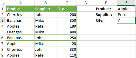
When you're learning something new, it's always a good idea to start with simple things. So, to begin with, let's define all the arguments for our SUMIFS formula:
- sum_range - C2:C9
- criteria_range1 - A2:A9
- criteria1 - "apples"
- criteria_range2 - B2:B9
- criteria2 - "Pete"
Now assemble the above parameters, and you will get the following SUMIFS formula:
=SUMIFS(C2:C9, A2:A9, "apples", B2:B9, "Pete")
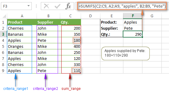
To refine the formula further, you can replace the text criteria "apples" and "Pete" with cell references. In this case, you won't have to change the formula to calculate the quantity of other fruit from a different supplier:
=SUMIFS(C2:C9, A2:A9, F1, B2:B9, F2)
Note. Both the SUMIF and SUMIFS functions are case-insensitive by nature. To get them to recognize the text case, please see Case-sensitive SUMIF and SUMIFS formula in Excel.
SUMIF vs. SUMIFS in Excel
Since the aim of this tutorial is to cover all possible ways to sum values by several conditions, we will discuss formula examples with both functions - Excel SUMIFS and SUMIF with multiple criteria. To use them correctly, you need to clearly understand what these two functions have in common and in what way they are different.
While the common part is clear (similar purpose and parameters), the differences are not so obvious, though very essential.
There are 4 major differences between SUMIF and SUMIFS:
- Number of conditions. SUMIF can evaluate just one condition at a time while SUMIFS can check for multiple criteria.
- Syntax. With SUMIF, the sum_range is the last and optional argument - if not defined, the values in the range argument are summed. With SUMIFS, sum_range is the first and required argument.
- Size of ranges. In SUMIF formulas, sum_range does not necessarily have to be of the same size and shape as range, as long as you have the top left cell right. In Excel SUMIFS, each criteria_range must contain the same number of rows and columns as the sum_range argument.
For example, SUMIF(A2:A9,F1,C2:C18) will return the correct result because the leftmost cell in the sum_range argument (C2) is right. So, Excel will make the correction automatically and include as many columns and rows in sum_range as there are in range.
A SUMIFS formula with unequally sized ranges will return a #VALUE! error.
- Availability. SUMIF is available in all Excel versions, from 365 through 2000. SUMIFS is available in Excel 2007 and higher.
Alright, enough strategy (i.e. theory), let's get into the tactics (i.e. formula examples : )
How to use SUMIFS in Excel - formula examples
A moment ago, we discussed a simple SUMIFS formula with two text criteria. In the same manner, you can use Excel SUMIFS with multiple criteria expressed by numbers, dates, logical expressions, and other Excel functions.
Example 1. Excel SUMIFS with comparison operators
In our fruit suppliers table, suppose, you want to sum all deliveries by Mike with Qty. 200 or more. To do this, you use the comparison operator "greater than or equal to" (>=) in criteria2 and get the following SUMIFS formula:
=SUMIFS(C2:C9,B2:B9,"Mike",C2:C9,">=200")
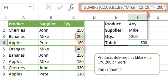
Note. Please pay attention that in Excel SUMIFS formulas, logical expressions with comparison operators should always be enclosed in double quotes ("").
We covered all possible comparison operators in detail when discussing Excel SUMIF function, the same operators can be used in SUMIFS criteria. For example, the following formula with return the sum of all values in cells C2:C9 that are greater than or equal to 200 and less than or equal to 300.
=SUMIFS(C2:C9, C2:C9,">=200", C2:C9,"<=300")
Example 2. Using Excel SUMIFS with dates
In case you want to sum values with multiple criteria based on the current date, use the TODAY() function in your SUMIFS criteria, as demonstrated below. The following formula sums values in column D if a corresponding date in column C falls within the last 7 days, including today:
=SUMIFS(D2:D10, C2:C10,">="&TODAY()-7, C2:C10,"<="&TODAY())
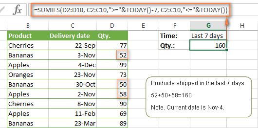
Note. When you use another Excel function together with a logical operator in the criteria, you have to use the ampersand (&) to concatenate a string, for example "<="&TODAY().
In a similar fashion, you can use the Excel SUMIF function to sum values in a given date range. For example, the following SUMIFS formula adds the values in cells C2:C9 if a date in column B falls between 1-Oct-2014 and 31-Oct-2014, inclusive.
=SUMIFS(C2:C9, B2:B9, ">=10/1/2014", B2:B9, "<=10/31/2014")
The same result can be achieved by calculating the difference of two SUMIF functions, as demonstrated in this example - How to use SUMIF to sum values in a given date range. However, Excel SUMIFS is much easier and more understandable, isn't it?
Example 3. Excel SUMIFS with blank and non-blank cells
When analyzing reports and other data, you may often need to sum values corresponding either to empty or non-empty cells.
| Criteria | Description | Formula Example | |
|---|---|---|---|
| Blank cells | "=" | Sum values corresponding to blank cells that contain absolutely nothing - no formula, no zero length string. | =SUMIFS(C2:C10, A2:A10, "=", B2:B10, "=")
Sum values in cells C2:C10 if the corresponding cells in columns A and B are absolutely empty. |
| "" | Sum values corresponding to "visually" blank cells including those that contain empty strings returned by some other Excel function (for example, cells with a formula like =""). | =SUMIFS(C2:C10, A2:A10, "", B2:B10, "")
Sum values in cells C2:C10 with the same conditions as the above formula, but includes empty strings. |
|
| Non-blank cells | "<>" | Sum values corresponding to non-empty cells, including zero length strings. | =SUMIFS(C2:C10, A2:A10, "<>", B2:B10, "<>")
Sum values in cells C2:C10 if the corresponding cells in columns A and B are not empty, including cells with empty strings. |
| SUM-SUMIF or SUM / LEN |
Sum values corresponding to non-empty cells, not including zero length strings. | =SUM(C2:C10) - SUMIFS(C2:C10, A2:A10, "", B2:B10, "")
=SUM((C2:C10) * (LEN(A2:A10)>0)*(LEN(B2:B10)>0)) Sum values in cells C2:C10 if the corresponding cells in columns A and B are not empty, cells with zero length strings are not included. |
And now, let's see how you can use a SUMIFS formula with "blank" and "non-blank" criteria on real data.
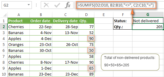
Suppose, you have an order date in column B, delivery date in column C and Qty. in column D. How do you find the total of products that have not been delivered yet? That is, you want to know the sum of values corresponding to non-empty cells in column B and empty cells in column C.
The solution is to use the SUMIFS formula with 2 criteria:
=SUMIFS(D2:D10, B2:B10,"<>", C2:C10,"=")
Using Excel SUMIF with multiple OR criteria
As noted in the beginning of this tutorial, the SUMIFS function is designed with AND logic. But what if you need to sum values with multiple OR criteria, i.e. when at least one of the conditions is met?
Example 1. SUMIF + SUMIF
The simplest solution is to sum the results returned by several SUMIF functions. For example, the following formula demonstrates how to find the total of products delivered by Mike and John:
=SUMIF(C2:C9,"Mike",D2:D9) + SUMIF(C2:C9,"John",D2:D9)
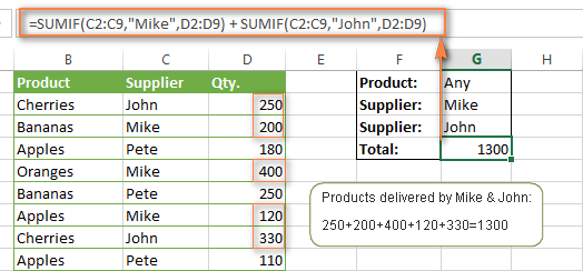
As you see, the first SUMIF function adds the quantities corresponding to "Mike", the other SUMIF function returns the amounts relating to "John" and then you add these 2 numbers.
Example 2. SUM & SUMIF with an array argument
The above solution is very simple and may get the job done quickly when there are only a couple of criteria. But a SUMIF + SUMIF formula may grow up enormously if you want to sum values with multiple OR conditions. In this case, a better approach is using an array criteria argument in the SUMIF function. Let's examine this approach now.
You can start by listing all of your conditions separated by commas and then enclose the resulting comma-separated list in {curly brackets}, which is technically called an array.
In the previous example, if you want to sum the products delivered by John, Mike and Pete, your array criteria will look like {"John","Mike","Pete"}. And the complete SUMIF function is SUMIF(C2:C9, {"John","Mike","Pete"} ,D2:D9).
The array argument consisting of 3 values forces your SUMIF formula to return three separate results, but since we write the formula in a single cell, it would return the first result only - i.e. the total of products delivered by John. To get this array-criteria approach to work, you have to use one more little trick - enclose your SUMIF formula in a SUM function, like this:
=SUM(SUMIF(C2:C9, {"John","Mike","Pete"} , D2:D9))
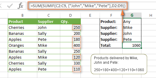
As you see, an array criteria makes the formula much more compact compared to SUMIF + SUMIF, and lets you add as many values as you like in the array.
This approach works with numbers as well as with text values. For instance, if instead of the suppliers' names in column C, you had supplier IDs like 1, 2, 3 etc., then your SUMIF formula would look similar to this:
=SUM(SUMIF(C2:C9, {1,2,3} , D2:D9))
Unlike text values, numbers needn't be enclosed in double quotes in array arguments.
Example 3. SUMPRODUCT & SUMIF
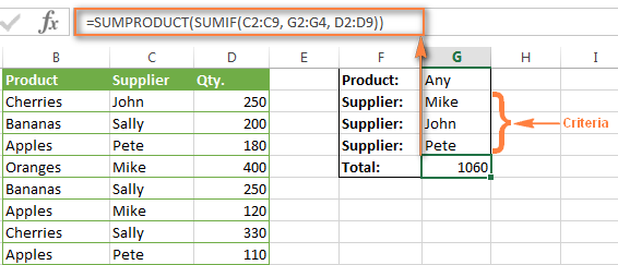
In case, your preferred way is to list the criteria in some cells rather that specify them directly in the formula, you can use SUMIF in conjunction with the SUMPRODUCT function that multiplies components in the given arrays, and returns the sum of those products.
=SUMPRODUCT(SUMIF(C2:C9, G2:G4, D2:D9))
Where G2:G4 are the cells containing your criteria, the suppliers' names in our case, as illustrated in the screenshot below.
But of course, nothing prevents you from listing the values in an array criteria of your SUMIF function if you want to:
=SUMPRODUCT(SUMIF(C2:C9, {"Mike","John","Pete"}, D2:D9))
The result returned by both formulas will be identical to what you see in the screenshot:
Excel SUMIFS with multiple OR criteria
If you want to conditionally sum values in Excel not simply with multiple OR conditions, but with several sets of conditions, you will have to use SUMIFS instead of SUMIF. The formulas will be very similar to what we've just discussed.
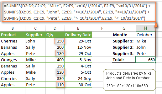
As usual, an example might help to illustrate the point better. In our table of fruit suppliers, let's add the Delivery Date (column E) and find the total quantity delivered by Mike, John and Pete in October.
Example 1. SUMIFS + SUMIFS
The formula produced by this approach includes a lot of repetition and looks cumbersome, but it is easy to understand and, most importantly, it works : )
=SUMIFS(D2:D9,C2:C9, "Mike", E2:E9,">=10/1/2014", E2:E9, "<=10/31/2014") +

SUMIFS(D2:D9, C2:C9, "John", E2:E9, ">=10/1/2014", E2:E9, "<=10/31/2014") +

SUMIFS(D2:D9, C2:C9, "Pete", E2:E9, ">=10/1/2014" ,E2:E9, "<=10/31/2014")
As you see, you write a separate SUMIFS function for each of the suppliers and include two conditions - equal to or greater than Oct-1 (">=10/1/2014",) and less than or equal to Oct 31 ("<=10/31/2014"), and then you sum the results.
Example 2. SUM & SUMIFS with an array argument
I've tried to explain the essence of this approach in the SUMIF example, so now we can simply copy that formula, change the order of arguments (as you remember it is different in SUMIF and SUMIFS) and add additional criteria. The resulting formula is more compact than SUMIFS + SUMIFS:
=SUM(SUMIFS(D2:D9,C2:C9, {"Mike", "John", "Pete"}, E2:E9,">=10/1/2014", E2:E9, "<=10/31/2014"))
The result returned by this formula is exactly the same as you see in the screenshot above.
Example 3. SUMPRODUCT & SUMIFS
As you remember, the SUMPRODUCT approach differs from the previous two in the way that you enter each of your criteria in a separate cell rather that specify them directly in the formula. In case of several criteria sets, the SUMPRODUCT function won't suffice and you will have to employ ISNUMBER and MATCH as well.
So, assuming that the Supplies Names are in cells H1:H3, Start Date is in cell H4 and End Date in cell H5, our SUMPRODUCT formula takes the following shape:
=SUMPRODUCT(--(E2:E9>=H4), --(E2:E9<=H5), --(ISNUMBER(MATCH(C2:C9, H1:H3,0))), D2:D9)
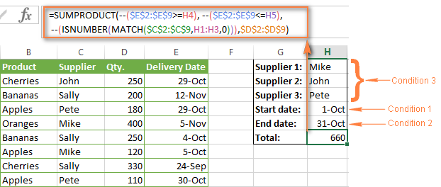
Many people wonder why use double dash (--) in SUMPRODUCT formulas. The point is that Excel SUMPRODUCT ignores all but numeric values, while the comparison operators in our formula return Boolean values (TRUE / FALSE), which are non-numeric. To convert these Boolean values to 1's and 0's, you use the double minus sign, which is technically called the double unary operator. The first unary coerces TRUE/FALSE to -1/0, respectively. The second unary negates the values, i.e. reverses the sign, turning them into +1 and 0, which the SUMPRODUCT function can understand.
I hope the above explanation makes sense. And even if it doesn't, just remember this rule of thumb - use the double unary operator (--) when you are using comparison operators in your SUMPRODUCT formulas.
Using Excel SUM in array formulas
As you remember, Microsoft implemented the SUMIFS function in Excel 2007. If someone still uses Excel 2003, 2000 or earlier, you will have to use a SUM array formula to add values with multiple AND criteria. Naturally, this approach works in modern versions of Excel 2013 - 2007 too, and can be deemed an old-fashioned counterpart of the SUMIFS function.
In the SUMIF formulas discussed above, you have already used array arguments, but an array formula is something different.
Example 1. Sum with multiple AND criteria in Excel 2003 and earlier
Let's get back to the very first example where we found out a sum of amounts relating to a given fruit and supplier:

As you already know, this task is easily accomplished using an ordinary SUMIFS formula:
=SUMIFS(C2:C9, A2:A9, "apples", B2:B9, "Pete")
And now, let's see how the same task can be fulfilled in early "SUMIFS-free" versions of Excel. First off, you write down all the conditions that should be met in the form of range="condition". In this example, we have two range/condition pairs:
Condition 1: A2:A9="apples"
Condition 2: B2:B9="Pete"
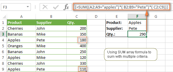
Then, you write a SUM formulas that "multiplies" all of your range/condition pairs, each enclosed in brackets. The last multiplier is the sum range, C2:C9 in our case:
=SUM((A2:A9="apples") * ( B2:B9="Pete") * ( C2:C9))
As illustrated in the screenshot below, the formula perfectly works in the latest Excel 2013 version.
Note. When entering any array formula, you must press Ctrl + Shift + Enter. Once you do this, your formula gets enclosed in {curly braces}, which is a visual indication that an array formula is entered correctly. If you try typing the braces manually, your formula will be converted to a text string, and it won't work.
Example 2. SUM array formulas in modern Excel versions
Even in modern versions of Excel, the power of the SUM function should not be underestimated. The SUM array formula is not simply gymnastics of the mind, but has a practical value, as demonstrated in the following example.
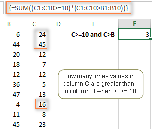
Suppose, you have two columns, B and C, and you need to count how many times column C is greater than column B, when a value in column C is greater or equal to 10. An immediate solution that comes to mind is using the SUM array formula:
=SUM((C1:C10>=10) * (C1:C10>B1:B10))
Don't see any practical application to the above formula? Think about it in another way : )
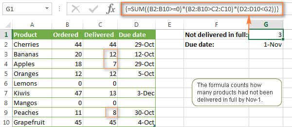
Suppose, you have the orders list like shown in the screenshot below and you want to know how many products have not been delivered in full by a given date. Translated into Excel's language, we have the following conditions:
Condition 1: A value in column B (Ordered items) is greater than 0
Condition 2: A value in column C (Delivered) in less than in column B
Condition 3: A date in column D (Due date) is less than 11/1/2014.
Putting the three range/condition pairs together, you get the following formula:
=SUM((B2:B10>=0)*(B2:B10>C2:C10)*(D2:D10<G2))
Well, the formula examples discussed in this tutorial have only scratched the surface of what Excel SUMIFS and SUMIF functions can really do. But hopefully, they have helped pointing you in the right direction and now you can sum values in your Excel workbooks no matter how many intricate conditions you have to consider.
 by
by
236 comments
I have an exported excel file. there is one column that is headed Job Status. Now there are about 6 to 8 different stages for the job. I want a formula that can sort this one column into the multiple columns by status. Can excel do that?
Hi! Based on your description, it is hard to completely understand your task. However, I’ll try to guess and offer you these guides: Excel FILTER function - dynamic filtering with formulas and Excel SORT function - auto sort data using formula.
Need some help please! Im new!
I want to sum B13:B18 if G23 is greater than 1 then * by G23 and sum B13:B18 if G23 is less than 1.
This is the formula i have so far.
=SUMIF(B13:B18,">"&G23)*G23(B13:B18,"<"&G23)
I am frustrated. I need my SUMIFS to work when the criteria is a cell reference. This formula does not seem to be nearly as useful if I have to type in the Criteria for each cell when I am copying the formula to multiple columns and rows that are referencing different data.
Thank you.
-Luke
Hey I am writing in googlesheet the formula but shows me error.
e.g
Date
Agency Name : Test1
Client Name : Test 1.1
Payable Amount: 1000euro
Office Margin: e.g 7%
Agency Margin: e.g 6%
Office Profit Amount: 70euro
Agency Profit Amount: 60euro
This is connected with a google form.
I want for to a formula to calculate total of agency profit amount: e.g name is Test 1 to find all test 1 in the google shit and the profit amounts and calculate them.
I use those but is writting error :=SUMIFS(H2:H30,B2:B30,"Test 1")
Hey Stelios,
Make sure column H contains numbers (remove the word euros and apply the currency format instead) and that your condition matches the Agency Name completely, e.g. Test1 and Test 1 are different values because of the space in-between.
For other nuances of SUMIFS in Google Sheets, please visit this article.
Hi, I have a data set with columns titled - Jan 1 2023 through Dec 31 2023. So each column is 1 day of the year up until Dec 31.
Then i have 11 rows - each with a different title which i call a code.
i.e., this is a snippet of my data set
Jan 1 Jan 2 Jan 3 Jan 4 ... Dec 31 2023
PED 0 3 2 6 3
SUS 0 0 0 1 2
BER 1 1 0 2 0
ETC.
I need to get a sum of each code per month on a separate tab. i.e., i'd have Jan through Dec month by month on a new tab in rows 2 to 13 and the different codes as column headers and then the sum of each code per month as the values within the table. I was trying to use a sumif but that won't work so i'm wondering what other function i can use??
Hi! To calculate the sum by condition in columns, you can use the SUMPRODUCT function. I recommend reading this guide: Excel SUMPRODUCT function with multiple criteria. To determine the month number, use the MONTH function.
For example:
=SUMPRODUCT((MONTH(B1:K1)=1)*B2:K2)
Hi Alex!
I am having trouble figuring out a conditional formula based on two words without a value. If I wanted to type formula that calculates the number of sold homes in oakmont how would that look for the example below?
A B
Oakmont Sold
Oakmont For Sale
Cedar Ridge Sold
Whispering Creek Sold
Oakmont Sold
Rock Creek sold
Oakmont for sale
Oakmont sold
Hi! If I understand your task correctly, count the number of "Oakmont sold" values. To do this, you can use the COUNTIF function and these instructions: COUNTIF function in Excel - count if not blank, greater than, duplicate or unique.
For example:
=COUNTIF(A1:A20,"Oakmont sold")
CAn we add value in excel ? like 1/1 + 1/1 = 2 /2
Your expression doesn't follow the rules of the mathematics.
Hi Alexander
I am trying to write a sumif formula that provides the grand total for a specific company, in a specific year and leave blank if there is nil income for that year. See example below, I want the sum total for Company A, for the year of 2023, provided the supplier code is the same, ignoring blanks. And what would the formula also be if I want to combine the income for 2022 and 2023?
Column A Column B Column C Column D Column E Column F
Supplier Product type Supplier Code Year 2022 Year 2023 Grand total
Company A Product 1 44 150 194
Company A Product 1 S7 9347 8421
Company A Product 2 44 34
Company B Product 1 55 273 265
Company B Product 2 S9 13722 7411
Company B Product 1 55 89
Company B Product 3 55
Company B Product 4 55 2
Company B Product5 55 56
Company C Product 1 S6 104591 79251
Company C Product 1 45 21743 5040
Company C Product 2 45
Company C Product 3 45 2015
Company C Product 4 45 342
Company D Product 1 S9 40895 42354
Company D Product 2 T30 142 155
Company E Product 1 11 9764
Hi! I hope you have studied the recommendations in the tutorial above. It contains answers to your question. For example, amount for 2022:
=SUMIFS(D2:D10,A2:A10,"Company A",C2:C10,1)
Analogously, find the amount for 2023 and then sum these results to find the amount for 2 years. Read above: Excel SUMIF with multiple criteria (OR logic).
PRODUCT SUPPLIER QTY.
CHERRIES JOHN 200
BANANA MIKE 350
APPLE PETE 180
ORANGE MIKE 400
BANANA JOHN 250
APPLE MIKE 120
CHERRIES JOHN 330
APPLE PETE 110
=SUM(SUMIF(A2:B9,{"APPLE","PETE"},C2:C9))
CAN i use it to find number of apples and nos of PETE PRODUCTS
Hi! I hope you have studied the recommendations in the tutorial above. To calculate the sum by multiple conditions, use the SUMIFS function:
=SUMIFS(C1:C8,A1:A8,"APPLE",B1:B8,"PETE")
Hi, I want to show the total amount for a certain product in a certain month/year (Column B, C, D, E)
RESULT SHOULD BE: The amount of Product 2 in Feb 2023
Column A Jan 2023 Feb 2023
Product 1 100 200
Product 2 50 38
Product 3 85 150
Hi, Alex! It works. Thank you so much.
Other one.
What if I want the total amount of Product2 from Jan2023-Feb2023
The same condition but I want the the TOTAL AMOUNT for Product2 from Jan2023-Feb2023
So, the result should be 88 (50+38)
Thanks!
Hi! To find the sum by condition for rows and columns, use the SUMPRODUCT function. For example,
=SUMPRODUCT(B2:M9*(A2:A9=N1)*((B1:M1=P1)+(B1:M1=P2)))
N1 = Product Name
P1, P2 = Column name ("Jan 2023", "Feb 2023")
Hi, Alex!
This formula is working
=SUMPRODUCT(B2:M9*(A2:A9=N1)*((B1:M1=P1)+(B1:M1=P2)))
Just want to clarify, I am using drop down list for Months.
I if will choose the month of JAN 2023 only for Product2, it multiplies the amount on the selected month.
So, if I have 50 For JAN 2023 it will become 100
By the way, I fixed 1 cell for JAN 2023 and I separated the dropdown list (JAN 22023, FEB 2023, MAR 2023)
Its like,
JAN 2023(fixed cell) + JAN 2023(Dropdown list)
JAN 2023(fixed cell) + FEB 2023(Dropdown list)
Hi, Alex!
This is the formula.
=SUMPRODUCT(G2:Q18*(A2:A18=R1)*((F1:Q1=R2)+(F1:Q1=R3)))
Whereas:
A2:A18 = List of Product
R1 = Product Name
R2 = JAN 2023
R3 = it can be from JAN 2023, FEB 2023, MAR 2023 . . . . . .
>If I want to calculate the total amount of PRODUCT 1 from JAN 2023 up to MAR 2023
>>If I want to calculate the total amount of PRODUCT 1 from JAN 2023 up to MAR 2023
Thanks!
Hi, Alex!
Unfortunately, the formula is not working, it leaves as zero (0) the sum product.
I even create new and simple data to execute the formula.
=SUMPRODUCT(B2:M9*(A2:A9=N1)*((TEXT(B1:M1,"mmm yy")=P1)+(TEXT(B1:M1,"mmm yy")=P2)))
Here are my data:
Column A2:A4 = Item1, Item2, Item3
Row B1:B3 = Jan 2023, Feb 2023, Mar 2023
Column:Row B2:D4 = are the data value (amount)
References:
Cell F1 = Item
Cell F2 = Month1
Cell F3 = Month2
Cell F4 = this cell will show the result
I hope these data would suffice for the formula.
Thanks!
Hi, Alex!
I found the correct formula.
=SUMPRODUCT(B2:M9*(A2:A9=N1)*(B1:M1>= P1)*(B1:M1<= P2))
Hi, Alex!
Thank you. I'll just try to find and explore the formula.
Thanks again.
Hi, Alex!
If I change the date
from: 01/01/2023
to: 01/03/2023
The result is not correct, as it will add only the data of Jan+Mar = 400
01/01/2023 = 100
01/02/2023 = 200
01/03/2023 = 300
How to sum if I change the date
from: 01/01/2023
to: 01/03/2023
result should be = 600
or
From: 01/02/2023
To: 01/12/2023
Apologies for the inconvenience.
Thank you!
Hi! I have already recommended to pay attention to the instructions on how to work with the SUMPRODUCT function: SUMPRODUCT formula with AND as well as OR logic.
Hi, Alex!
B1:B3 - Text or date?
>these are date 01/01/2023
F2, F3 - Text or date?
>these are date also, it was a dropdown list and the source are from B1:B3
What is written in F2?
>01/01/2023
Here is the sum by rows and columns formula for your data:
=SUMPRODUCT(B2:M9*(A2:A9=N1)*((B1:M1=P1)+(B1:M1=P2)))
Hi! You use text values to represent months in the column headers. Therefore, you cannot use the time interval "from - to". You must specify each month name separately. For 3 months you need 3 cells.
Hi, Alex!
The formula below is working, but how can I sum the amount from JAN 2023 to MAR 2023 or FEB 2023 to MAR 2023?
=SUMPRODUCT(B2:M9*(A2:A9=N1)*(TEXT(B1:M1,"mmm yy")=P1))
I tried the formula below, but if I change FEB 2023 to MAR 2023 it will not be summed the amount.
=SUMPRODUCT(B2:M9*(A2:A9=N1)*(TEXT(B1:M1,"mmm yy")=P1))+(TEXT(B1:M1,"mmm yy")=P2))
=SUMPRODUCT(B2:M9*(A2:A9=N1)*(TEXT(B1:M1,"mmm yy")=P1))*(TEXT(B1:M1,"mmm yy")=P2))
Thanks,
Hi! To calculate the amount by product for two months, the formula might look like this:
=SUMPRODUCT(B2:M9*(A2:A9=N1)*((TEXT(B1:M1,"mmm yy")=P1)+(TEXT(B1:M1,"mmm yy")=P2)))
Hi, Alex!
The headers are dates literally, it just formatted as (MMM YYYY)
The formula below is working correctly for FEB 2023 only
=SUMPRODUCT(G2:Q18*(A2:A18=R1)*((F1:Q1=R2)+(F1:Q1=R3)))
Whereas:
A2:A18 = List of Product
R1 = Product Name
F1:Q1 = MMM YYYY (Date)
R2 = JAN 2023
R3 = it can be from JAN 2023, FEB 2023, MAR 2023 . . . . . .
>How to calculate the total amount of PRODUCT 1 from JAN 2023 up to MAR 2023
>> How to calculate the total amount of PRODUCT 1 from JAN 2023 up to FEB 2023
>>> How to calculate the total amount of PRODUCT 1 from FEB 2023 up to MAR 2023
Thanks!
Hi! Use the TEXT function to convert the date to text and compare to the criteria.
=SUMPRODUCT(B2:M9*(A2:A9=N1)*(TEXT(B1:M1,"mmm yy")=P1))
Hi! Since you need to find only one value, I recommend using these instructions with examples: INDEX MATCH MATCH to lookup in rows and columns. I hope it’ll be helpful.
Hi,
i have SAP product codes which are 19 in digits which are note reading by "SUMIFS" while considering multiple conditions like "900000002831022000".
If I'm decreasing its digits lesser than 19, its working perfectly.
Could you please assist on it.
Hi! Excel does not work with numbers longer than 15 digits. Write such long numbers as text. Maybe this article will be helpful: How to convert numbers to text using Excel TEXT function and other options.
Much appreciated.
Hello,
What if I want to count the bananas from both suppliers John and Mike? Do you have a better solution than :
=SUMIFS(C2:C9, A2:A9, "Bananas", B2:B9, "John") + SUMIFS(C2:C9, A2:A9, "Bananas", B2:B9, "Mike") ?
How can I put option A or Option B or Option C in the same criteria in that case that would apply to B2:B9?
Thank you!
Hi! If you read carefully, the last paragraph of this article has the answer to your question. Here is an example of the formula:
=SUM((A2:A10="Bananas")*((B2:B10="John")+(B2:B10="Mike"))*C2:C10)
HI, I want to use SUMIFS, and the cells in the range that I want to consider already have a formula (IF), but the SUMIFS is not considering those values. How can I do? thanks!
Hi! The SUMIFS function does an excellent job of counting cells with formulas. What is important is what values these formulas return.
Hi
I have data with multiple units (i.e, Kg, Pcs, Nos, etc). Some items may appear in multiple units. for example, sometimes I sell an item in pcs and sometimes in Kg. So, to get how much qty I sold in a month what will be the equation?
Hi! To sum values with the same unit of measurement, use the SUMIFS function. Read article above.
Hi, I have an issue in defining a formula to sum different rows in a matrix based on different filters:
Date 29/12/2022 29/01/2023 29/01/2024 29/01/2025
Flow -189.110,0 5.890,0 5.890,0 5.890,0
Key 122022 12023 12024 12025
Date 29/12/2022 16/09/2023 16/09/2024 16/09/2025
Flow -175.723,4 6.317,5 6.317,5 196.317,5
Key 122022 92023 92024 92025
I have a matrix like this (sorry for the format): I have to define a formula to sum the "Flow" row based on the key field. Say I have to build a cash flow report, so I have all the month for a year and for each month I have to sum the different flows through the "Key" row. Is there a formula without repeating sumif for all the lines?
Many thanks for any help.
Alberto
Hi! SUMIFS function cannot sum over columns. So try the SUMPRODUCT function. I'm not quite sure how your data is organized, but the formula might look something like this:
=SUMPRODUCT((B3:N3=12022)*(MONTH(B1:N1)=1)*(YEAR(B1:N1)=2023)*B2:N2)
If this is not what you wanted, please describe the problem in more detail.
How do I ask Excel to give a sum or count for data like the below? For the below, I would want a count of 1 because all activity occurred roughly at the same time. I don't want to count each row as its own instance but rather count them as one singular event.
StationName TransactionDateTime TransactionType MedID DrawerSubDrawerPocket Quantity
G3SE 1/1/2023 9:21 Refill 64573 Drw 3.14-Pkt 2 3
G3SE 1/1/2023 9:21 Refill 64573 Drw 3.14-Pkt 1 3
G3SE 1/1/2023 9:21 Refill 64573 Drw 3.14-Pkt 3 0
G3SE 1/1/2023 9:22 Refill 64573 Drw 3.9-Pkt 2 1
G3SE 1/1/2023 9:22 Refill 64573 Drw 3.9-Pkt 4 0
G3SE 1/1/2023 9:22 Refill 64573 Drw 3.9-Pkt 1 2
G3SE 1/1/2023 9:22 Refill 64573 Drw 3.9-Pkt 3 0
Hi! Set the time interval at which all events can be counted as one. Use these guidelines: Excel SUMIFS date range formula - sum if between two dates. Pay attention to the following paragraph of this article: Sum if between two dates and another criteria.
Hi All,
From the example:
=SUM(SUMIF(C2:C9, {"John","Mike","Pete"} , D2:D9))
If i want to store the set of criteria in a cell how would i do that, when swap the criteria for a cell, and paste the values into the cell it does not work, so:
=SUM(SUMIF(C2:C9, A1, D2:D9))
In cell A1 - {"John","Mike","Pete"}
or "John","Mike","Pete"
Any ideas?
Hi! The SUMIF function cannot get an array of values from a cell. You can use a cell reference that contains only one value.
For example,
=SUM(SUMIF(C2:C9, A1, D2:D9),SUMIF(C2:C9, A2, D2:D9))
where A1 - John. A2 - Mike
You can use the TEXTSPLIT function which will return an array of text values from a cell using a separator. For example,
=SUM(SUMIF(C2:C9,TEXTSPLIT(A1," "),D2:D9))
where A1 - John Mike Pete
Been Trying this out since Wednesday, and you just solved the puzzle.
Thanks alot sir!
Alexander Trifuntov (Ablebits Team)
Hi,
I want to sum Hours!C8:C373 (this is employee time off hours)
If Hours!D8:D373 (this is the time off ID code)
= Summary!D4 (this is the time off ID I'm looking for)
And Summary!C5 (this is the employee name whose info I'm looking for)
= Hours!C7 (employee name and column header)
I tried this =IF(C5=Hours!C7,SUMIF(Hours!$D$8:$D$373,F$4,Hours!$C$8:$C$373),"") on the Summary sheet and it works.
Is there a better way? Thanks
Hi! You can use SUMPRODUCT instead of SUMIF, but you will get the same result. The formula might look something like this:
IF(C5=Hours!C7,SUMPRODUUCT((--(Hours!$D$8:$D$373=F$4))*Hours!$C$8:$C$373),"")
For more information, please read: Excel SUMPRODUCT function with multiple criteria.
IS the following formula correct:
=SUMIFS(D60:D1549,("4" ,TEXT(D60:D1549,"mm")))
please write the correct one.
Thanks so much.
Hi! The SUMIFS function cannot use other functions or expressions as arguments. Only values or cell references can be arguments to this function. I can't fix the formula as I don't know what you want to do.
Hello, Please help and thank you in advance!!
=IF(D4:D7="KHR",E4:E7/4000,SUMIF(F4:F7,"Red",E4:E7))
Hi! I don't know what you want to do, but note that D4:D7="KHR" returns an array of 4 values. Your formula cannot work.