Want to know how many characters there are in a certain cell? This tutorial will help you choose an Excel formula for character count best suited for your particular case.
Initially, Excel was designed to work with numbers. Fortunately, the developers of this helpful application didn't forget about text. Below, you'll find a number of formulas for counting characters in Excel. Just look through the examples and see which one best suits your needs.
Here are the cases we are going to cover:
Excel formula to count the number of characters in a cell
First things first, let's solve the most common case. To find how many characters there are in an Excel cell, the formula is as simple as:
For example, to count characters in each cell of column A beginning in A3, this is what you need to do:
- Enter the below formula in any empty cell in row 3:
=LEN(A3) - Double-click the fill handle to get the formula copied across the whole column.
Done!
Feel free to use this formula each time you need to count the number of characters in a string.
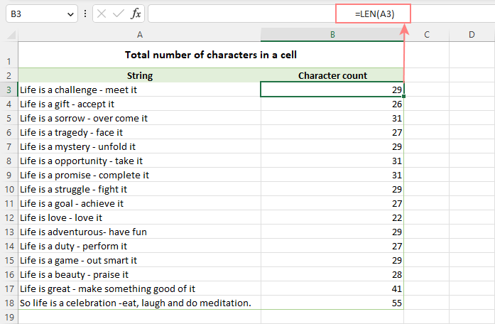
Note. Please pay attention that the Excel LEN function counts absolutely all characters in a cell, including letters, numbers, punctuation marks, special symbols, and all spaces (leading, trailing and spaces between words).
Count characters in a range of cells
To get the total of characters in an Excel range, you can use the LEN function together with SUMPRODUCT:
And your real-life formula may look similar to this:
=SUMPRODUCT(LEN(A3:A18))
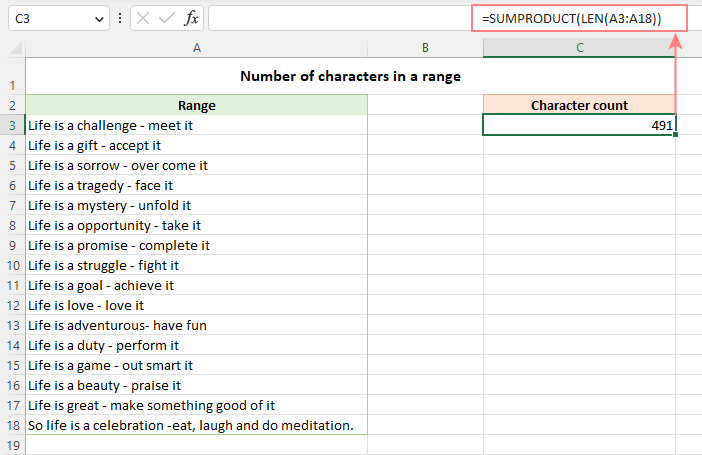
Another way to count all characters in a range is using LEN in combination with the SUM function:
=SUM(LEN(A3:A18))
Unlike SUMPRODUCT, the SUM function does not process arrays by default, so you need to press Ctrl + Shift + Enter to turn it into an array formula in Excel 2019 and earlier. In Excel 365 and 2021, it works as a regular formula due to inbuilt support for dynamic arrays.
How this formula works:
The logic is very simple. The LEN function calculates the string length for each individual cell in the specified range and returns an array of numbers. And then, SUMPRODUCT or SUM adds up those numbers and returns the total character count.
How to count specific characters in a cell
To find out how many times a given character appears in a cell, the generic formula is:
Suppose you maintain a database of items where each item type has its own unique identifier. And each cell contains several items separated by comma, space, or any other delimiter. The task is to get the number of occurrences of a certain unique identifier in each cell.
Assuming the list of items is in column A beginning in A3, and the target character is in column B in the same row, the formula is as follows:
=LEN(A3) - LEN(SUBSTITUTE(A3, B3, ""))
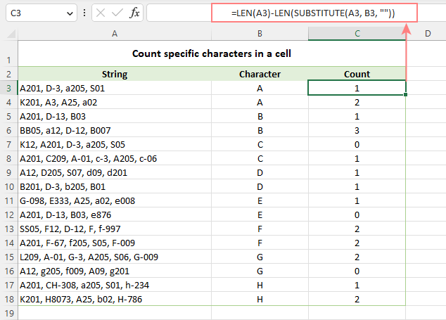
Note. Excel's SUBSTITUTE is a case-sensitive function, and therefore the above formula treats uppercase and lowercase letters as different characters. For example, cell A4 in the screenshot above contains one occurrence of "a" and two occurrences of "A". The formula counted only the uppercase "A" and returned 2 as the result.
How this formula works:
To understand the formula's logic, let's break it down into smaller parts:
- First, you find the total string length in cell A3 with:
LEN(A3) - Then, you remove all occurrences of the letter "A" in A3 by replacing it with an empty string:
SUBSTITUTE(A3, "A", "") - The next step is to find the string length without the letter "A":
LEN(SUBSTITUTE(A3, "A", "")) - Finally, you subtract the length of the string without "A" from the total length string:
LEN(A3) - LEN(SUBSTITUTE(A3, B3, ""))
As the result, you get the count of "removed" characters, which is the number of occurrences of that particular character in the cell.
Case-insensitive formula to count letters in Excel cell
When counting letters in Excel cells, you may sometimes need a formula that ignores the letter case. To make such a formula, use the UPPER function inside SUBSTITUTE to convert a given letter to uppercase before running the substitution.
For example, to count both "A" and "a" in cell A3, use this formula:
=LEN(A3) - LEN(SUBSTITUTE(UPPER(A3), "A", ""))
The LOWER function will also do:
=LEN(A3) - LEN(SUBSTITUTE(LOWER(A3), "a", ""))
A slightly more complex way is using nested SUBSTITUTE functions:
=LEN(A3) - LEN(SUBSTITUTE(SUBSTITUTE (A3, "A", ""), "a", "")
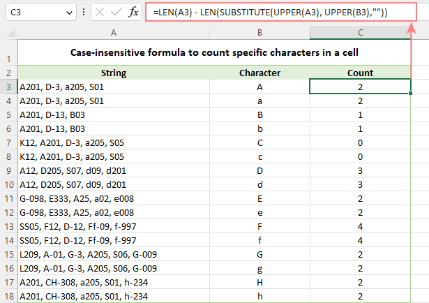
In our data set, the letters to be counted are input in column B, so we convert both the source cell and the cell containing the character to uppercase:
=LEN(A3) - LEN(SUBSTITUTE(UPPER(A3), UPPER(B3),""))
And this works beautifully irrespective of the target letter's case:
How to count certain text/substring in a cell
If you want to know how many times a certain combination of characters appears in a given cell (e.g. "C2" or "C-2" or "cat"), then divide the characters count by the length of the substring.
Case-sensitive formula:
=(LEN(A3) - LEN(SUBSTITUTE(A3, B3, ""))) / LEN(B3)
Case-insensitive formula:
=(LEN(A3)-LEN(SUBSTITUTE(UPPER(A3), UPPER(B3),""))) / LEN(B3)
Where A3 is the original text string and B3 is the substring to count.
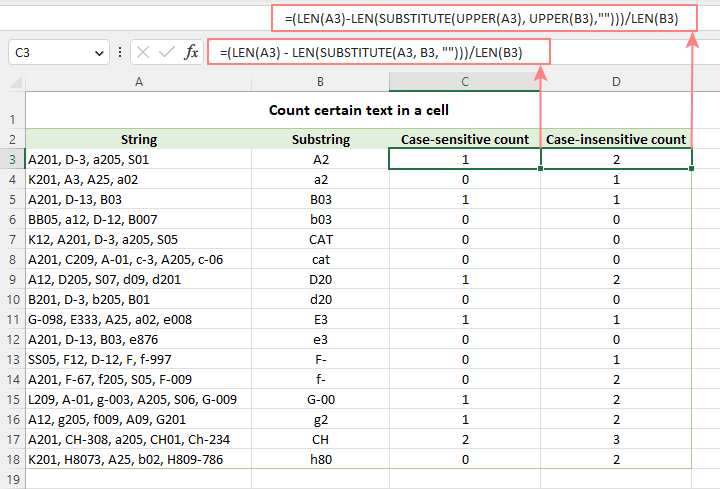
For the detailed explanation of the formula, please see How to count specific text / words in a cell.
How to count specific characters in a range
Knowing a formula for counting certain characters in a single cell, it's quite easy to modify it a little further to count the number of occurrences of a given character in several cells. For this, just place the LEN formula inside the SUMPRODUCT function that can handle arrays:
For example, to get to know how many times the character in D2 occurs in the range A3:A18, the formula is:
=SUMPRODUCT(LEN(A3:A18) - LEN(SUBSTITUTE(A3:A18, D2, "")))
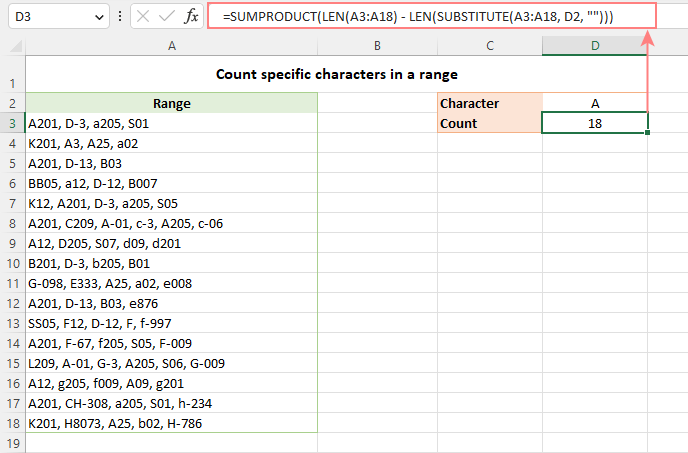
Instead of SUMPRODUCT, you can also use SUM:
=SUM(LEN(A3:A18) - LEN(SUBSTITUTE(A3:A18, D2, "")))
But this formula requires pressing Ctrl + Shift + Enter because, in all versions other than Excel 365 and 2021, SUM can handle arrays only in an array formula.
How this formula works:
The SUBSTITUTE function replaces all occurrences of a given character ("A" in this example) with an empty string ("").
The text string returned by SUBSTITUTE is served to the LEN function so it calculates the string length without A's.
The string length without A's is subtracted from the total length of the original string. The result is an array of character counts per cell.
Finally, SUMPRODUCT sums the numbers in the array and returns the total character count in the range.
Case-insensitive formula to count letters in a range
To create a case-insensitive formula for counting specific characters in a range, follow the same approaches that we used for counting certain letters in a cell regardless of the text case.
Use the UPPER function and supply an uppercase letter:
=SUMPRODUCT(LEN(A3:A18) - LEN(SUBSTITUTE(UPPER(A3:A18), "A", "")))
Use the LOWER function and supply a lowercase letter:
=SUMPRODUCT(LEN(A3:A18) - LEN(SUBSTITUTE(LOWER(A3:A18), "a", "")))
Nest a couple of SUBSTITUTE functions one into another:
=SUMPRODUCT(LEN(A3:A18) - LEN(SUBSTITUTE(SUBSTITUTE((A3:A18), "A", ""), "a", "")))
In the character of interest is input in a predefined cell, UPPER or LOWER will work equally well:
=SUMPRODUCT(LEN(A3:A18) - LEN(SUBSTITUTE(UPPER(A3:A18), UPPER(D2), "")))
Or
=SUMPRODUCT(LEN(A3:A18) - LEN(SUBSTITUTE(LOWER(A3:A18), LOWER(D2), "")))
The below screenshot shows it in action:
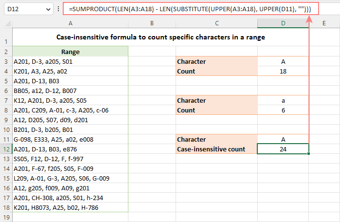
How to count certain text / substring in a range
To count the number of occurrences of certain text in a range, use this generic formula:
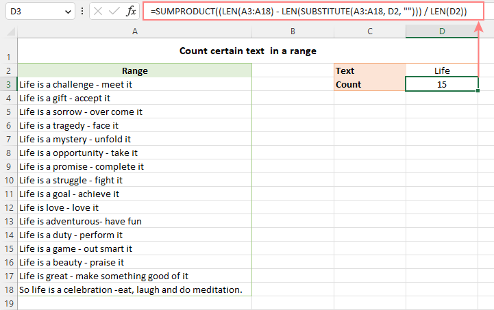
For example, to count the number of times the word "Life" appears in the range A3:A18, the formula is:
=SUMPRODUCT((LEN(A3:A18) - LEN(SUBSTITUTE(A3:A18, D2, ""))) / LEN(D2))
Excel character limits for cells
Microsoft Excel has a limitation on the number of characters that can be entered in a cell. If you have worksheets with large amount of text data, you may find the following information helpful.
- The total number of characters that a cell can contain is 32,767.
- A cell can only display 1,024 characters. At the same time, the Formula bar can show all 32,767 symbols.
- The maximum length of a formula is 8,192 characters in Excel 2007 and higher (1,014 in Excel 2003).
Please consider the facts when you are going to merge or import data from an external source.
These are the best practices for counting characters in Excel. For first-hand experience, you can download a sample workbook and check out a list of related resources at the end of the page. Thank you for reading and hope to see you soon!
Practice workbook for download
Count characters in Excel - formula examples (.xlsx file)
 by
by
76 comments
Hello,
Please help with formula.
How may i count how many letters are in specific range
i.e.
a b c
a b a a c a 4 1 1
a b c c b c 1 2 3
Hi! I recommend that you read the article carefully and pay attention to this section: Count characters in a range.
Those abc in the first row are above numbers 411 in table
i have to sum only letters. So the result i.e. is:
4 letters a in fist row
1 letter b in first row
1 letter c in first row
1 letter a in second row
2 letters b in second row
3 letters c in second row
How would I count the no of characters to the letter x
Eg 123x546789= 6
Hi! If I understand the question correctly, you can split a text string into individual characters using the MID function. Then you can use the MATCH function to find the position number of the character that you need to find.
=MATCH("x",MID(A1,ROW(A1:A20),1),0)
To find the number of characters before:
=MATCH("x",MID(A1,ROW(A1:A20),1),0)-1
To find the number of characters after:
=LEN(A1)-MATCH("x",MID(A1,ROW(A1:A20),1),0)
LEN function calculates the length of a text string.
How to count no of digits of a number
in a cell.
e.g: if cell A1 contains a no say 2024060302414806.
I need a formula to give me count of digits as 16.
Hi! Use MID function to extract each character from the text. Mathematical operation on letters returns an error, double minus on numbers returns a number. Count values and ignore errors using COUNT function. To count the quantity of digits in the text try this formula:
=COUNT(--MID(A1,ROW(A1:A50),1))
Hi!
I'm currently using a dropdown list to force a choice of 7 options 1, x , 2, 1x, x2, 12, 1x2.
And to get the most choosen value I've used: =INDEX(I2:N2;MODE(IF(I2:N2"";MATCH(I2:N2;I2:N2;0)))).
But the thing is it is counting 1x as one result, but I would rather it counted it as 1 "1" and one "x"
so for example if two people made their choices and chose 1x and 1, the above formula would show "1x" (as it is a tie but it is first in the column). I would like it to show 1 (count it as two number 1, and one X) instead. Is this possible?
Hello!
If I got you right, the formula below will help you with your task:
=INDEX(MID(CONCAT(I2:N2),ROW(1:20),1), MODE(IF(MID(CONCAT(I2:N2),ROW(1:20),1)<>"", MATCH(MID(CONCAT(I2:N2),ROW(1:20),1), MID(CONCAT(I2:N2), ROW(1:20),1),0))))
Hi again,
This was exactly what I was looking for, works like a charm!
Thanks a bunch!
Hi Again!
Is it possible to as well (in another cell) get the 2nd most chosen value?
I tried to get it through the below formula:
=INDEX(MID(CONCAT(I2:N2);ROW(1:20);1); MODE(IF(MID(CONCAT(I2:N2);ROW(1:20);1)"")*(MID(CONCAT(I2:N2);ROW(1:20);1);INDEX(MID(CONCAT(I2:N2);ROW(1:20);1);MODE(IF(MID(CONCAT(I2:N2);ROW(1:20);1)"";MATCH(MID(CONCAT(I2:N2);ROW(1:20);1);MID(CONCAT(I2:N2); ROW(1:20);1);0))))
But I'm definitely doing something wrong, and I realized I'm a bit above my knowledge level now as I don't fully comprehend the formula you helped me with (It works great though).
What I'm trying to achieve when it all is finished is one cell showing the most common value (as you helped me with above) and one cell showing the 2nd most common value and the difference between them, say If i have 5 "1" and 3 "x", The main goal is to get one (preferable) or two cells showing "X 2" as 5 - 3 = 2 (the difference).
I'm trying to read up on the above functions, but so far I'm not even sure if it is possible to do like I intended.
I am trying to exclude certain words/Text from the Filter. How do I uniquely count a column but ignore one repetitive entry.
Hello!
Use the SUMIFS function to calculate the sum of a column based on conditions. Here is a guide with examples: Excel SUMIFS and SUMIF with multiple criteria.
I should add, this is similar to ignoring spaces etc. I want to ignore a word, using COUNTA(UNIQUE(FILTER( ))
Hello
I am trying to get the bifurcation of categories of students in excel. but I can't get the result using the exists formulas in excel. Kindly help me to get it resolved.
The Problem is: In an attendance book there are 3 categories of students. the name of category is clearly mentioned in front of the name of the students. If there are 50 students in a classroom few students are belong to SC category, few are ST category and rest are General category. The attendance is marked P as present and A as Absent. Based on their categories, I have to calculate, how many SC category students are presented and in the same way other two categories.
Hi!
If you want to count values by two criteria, then use the COUNTIFS function.
An example formula for your data is
=COUNTIFS(A1:A10,"ST",C1:C10,"P")
Hi,
I am using EXCEL 2007(IF FORMULA APPLICABLE IN LATEST VERSIONS OF EXCEL I CAN SWIFT TO NEW VERSIONS)
i need in a following data of some persons, if in case they are continuously "P", then at 7th place i have to note as "PW"
DAYS
SNO NAMES 1 2 3 4 5 6 7 8 9 10 11 12 13 14 15 16 17 18 19 20 21 22 23 24 25 26 27 28 29 30
1 JACK P P P P P P P P A P P P P P A P P P P P P P P P P P P P A A A P P P P P P P P P
2 JILL P P P P A A P P P P P P P P P P P P P A P P P P P P P P P P P P P P P A P P P P
3 JOHN P P P P P P P A A P P P A P A P P P P P P P P P P P P P A P P P P P A P P P P P
AFTER applying formula i want to get like this
1 JACK P P P P P P PW P A P P P P P P A P P P P P P PW P P P P P P A A A P P P P P P PW P P
2 JILL P P P P A A P P P P P P PW P P P P P P A P P P P P P PW P P P P P P PW P A P P P P
3 JOHN P P P P P P PW A A P P P A P A P P P P P P PW P P P P P P A P P P P P A P P P P P
KINDLY SHARE FORMULA to my mail id IF AVAILABLE(saisandeepnagari@hotmail.com), BY MANUALLY CHECKING AND TYPING, TIME TAKING PROCESS FOR LARGE DATA IN EXCEL
Hi!
If each line is text, then you can use the SUBSTITUTE function to find and replace characters.
=SUBSTITUTE(A2,"P P P P P P P","P P P P P P PW")
If each character is written in a separate cell, then you can only replace characters using a VBA macro.
Dear Sir,
Each P is written in separate Cell,
Kindly explain how to replace characters in VBA macro.
KINDLY SHARE FORMULA to my mail id IF AVAILABLE(saisandeepnagari@hotmail.com)
Hi!
You can concatenate separate cells into one string, as described in this guide: TEXTJOIN function in Excel - easy way to merge text from multiple cells.
For example,
=TEXTJOIN(" ",FALSE,A1:H1)
Then use the formula recommended for you to replace the characters. Then split the text into cells again. Read detailed instructions here: How to split cells in Excel: Text to Columns, Flash Fill and formulas.
I want to count the letter of alpha numeric how many times itbwaa repeated in the sheet. Can you provide the answer.
Ex :
column a, row 1 : 1a,3b,2c
Column a, row 2 : 2a,3b,5d
Means here if if we use formula means when we search for 3b means the count should be 2.
Can you suggest how to write the code.
Hello!
Count the number of occurrences of certain text in a range - read above
Thanks for the reply,
I tried with same code in open office but it's not working it's showing #value instead of result. Is there any conflicts with "," in the column when we are searching with the formula which you gave. Actually my query is to find the alphanumeric ex : 2a how many times it's repeated along with another alphanumeric from column a row 1 to row 6
1a,2a,3a,5d
2c,4d,2a,7b
2a
3c,5d,6c
8a,11b
2a,10b
Now I want to search the letter 2a how many times repeated and it should be count even we are having "," in a cell.
My answer it should be 4 when we search from column A1:A6, similarly if we search for another alphanumeric also I need to get the result.
Hello!
Please try the following formula:
=SUM(--(ISNUMBER(FIND("2a",A1:A6,1))))
Ok I will and I will let u know.
Tried with the formula which you gave but not getting.
Is there any other formula...
Condition Report Type Sale
Condition 01 Sales Report 14
Condition 02 My Report 43
Condition 03 Report 25
Condition 04 Sales 76
Condition 05 Report 35
Condition 06 James's Report 85
Condition 07 Total 11
Condition 08 Report From my Boss 8
Condition 09 Not a Report 43
Count how many times words end with letter RT and contains 6 letters in Column C.
Hello Gajanan!
If I got you right, the formula below will help you with your task:
=SUM(--(RIGHT(C1:C10,2)="RT"))
=SUM(--(LEN(C1:C10)=6))
I hope it’ll be helpful.
how i count "p" in row in work sheet
Hi!
Change the formula that is recommended in this article
=SUM(LEN(A1:N1)-LEN(SUBSTITUTE(A1:N1,"p","")))
123456789 text box no how to count plz tell me formula
result 45 how
Hi Guys,
I am not getting solve question that how will count this is.
please find below this question.
22pcs 5kg
15pcs 8kg
16pcs 10kg
65pcs 12kg
How will i count and sum please assist me.
Thanks and Regards,
Sujan
Sujan:
Enter "pcs" and "kg" in cells C62 and D62. These will be the headers.
Enter the data in A48:A57. The formula is case sensitive so be sure the data matches the caps in the headers.
In C63 enter =SUM(IF(ISNUMBER(FIND(C62,$A$48:$A$57)),VALUE(LEFT($A$48:$A$57,FIND(C62,$A$48:$A$57)-1)),0))
then with the cursor in the formula bar in the formula click the CTRL Shift Enter keys at the same time. This is an array formula so you need to tell Excel to evaluate it as an array. When you enter the formula and then in the formula bar you put the cursor in the formula and click the CTL SHIFT ENTER keys it will put curly brackets around the formula which indicates to Excel that this is an array.
When the value appears in C63 copy the formula over to D63.
As you enter more data in the A range be sure to change the second cell address to match the last cell in the range. Right now the range is A48 to A57. If you add more data change the A57 to another cell address. Remember, there are three places in the formula for that range.
Thanks Doug.
But is it possible to do sum without transferring text to the other column
I don't want the result like below:
20 cow
60 Cow
70 Cow
150
I want the result of sum like this:
20Cow
60Cow
70Cow
150Cow
Pls help how can I do.
Paul:
As is often the case in Excel, there are a couple of different ways to get to where you want to go.
Check out this article here on AbleBits for the explanations and examples of several ways to do what you're trying to do.
https://www.ablebits.com/office-addins-blog/excel-if-cell-contains-count-sum/
I want to do sum for the following which contain number & Words
20 cows
60 Cows
70 cows
Result should be 150 or 150 cows.
But if I use auto sum it does not work. How can I do it? Pls help me.
Paul:
Split the numbers from the words using Text-to-Columns.
Highlight the cell, go to Data then choose Text-to-Columns and follow the prompts. After the words and numbers have been separated into their own cells you can use =Sum on the cells that contain numbers.
Dear support,
I have big sheet.there is contain text id..when i filter sheet i cannot get total count of filtered text...
Hello,
If I understand your task correctly, please try the following formula:
=SUBTOTAL(103,A2:A100)
Hope it will help you.
Hi,
I have data look like this below
R0754117
R0658417
P0256413
PX5698452
SO2584696
How do I do the countif wihtout the numeric? I just want to know how many count for R, P, PX and SO? Your help is appreciated. Thanks!
FIRST APPLY THIS
=LEFT(TEXT CELL,MIN(FIND({1,2,3,4,5,6,7,8,9,0},TEXT CELL&"1234567890")-1))
IT'S GIVE U A NUMBER, AFTER THAT U WILL COPY THIS FORMULA AND PASTE IN THIS
=SUBSTITUTE(TEXT CELL, LEFT(TEXT CELL,MIN(FIND({1,2,3,4,5,6,7,8,9,0},TEXT CELL&"1234567890"),"")
I HOPE U WILL BE GET YOU ANSWER
Hi, Amanda,
if the data is situated in A1:A5, use the following formula to count the number of cells with R at the beginning of the cell:
=COUNTIF(A1:A5,"R*")
To count the rest of the values simply change R in the formula to other letters.
You can read more about COUNTIF function on our blog post here.
How to Sum of this data
4 hours
8 hours
3 hours
6 hours
=sum(?????
Hello, Yogender,
at first, please make sure that the Time format is applied to your values.
Then, if the data starts in A2, use the following formula:
=SUM(A2:A5)
If the values are not in the cells use the following:
=SUM(TIME(4,0,0),TIME(8,0,0),TIME(3,0,0),TIME(6,0,0))
Hi Maria,
Hope you are doing well, I am a basic excel user, I am handling an excel work book in 2016 version, I've got a query as follows:
I have 9 worksheets in an excel book and a specific column in each sheet which displays a series of reference numbers as:
GAD5-CDC-T2-349-230315-DWG-PP-STR-0114-0
GAD5-MGM-T2-349-230315-DWG-PP-STR-0114-0
GAD5-CDC-T2-349-230315-DWG-SD-STR-0114-0
GAD5-MGM-T2-363-250315-DWG-PP-STR-0119-0
GAD5-CDC-T2-363-250315-DWG-DD-STR-0119-0
GAD5-CDC-T2-363-250315-DWG-BD-STR-0119-0
GAD5-CDC-T2-259-51-050515-DWG-FD-S-0233-00
GAD5-CDC-T2-259-51-050515-DWG-TD-S-0233-00
GAD5-MGM-T2-259-51-050515-DWG-LD-S-0233-00
GAD5-MGM-T3-119-25-DDS-ST-1568-02
GAD5-MGM-T3-119-25-DDS-RT-1568-02
GAD5-MGM-T3-119-25-DDS-OT-1568-02
and so on, Please note: these numbers are not following any sequence. I want to count the number of times the second last series of number is appearing. In this Instance
0114 is 3 times
0119 is 3 times
0233 is 3 times &
1568 is 3 times
I want to count this by a formula and get the result in any other cell as a counter. I'll appreciate if you could help me in this please.
Hi Syed,
You should use the following formula to count all cells with "0114":
=CONCATENATE("0114 is ", SUMPRODUCT((MID(A1:A12, FIND("-", A1:A12, LEN(A1:A12) - 8) + 1, 4) = "0114") * 1), " times")
You can change this formula and use it to count cells with "0119", "0233", etc.
hey i want to do the validation of PAN no. i.e. in between first five char are alfabets, next four are numeric & last one is also alfabet. its total 10 digit of no. so how can I check multiple PAN nos. at one tym. please tell me the formula.
Hi dinesh,
You should use the following formula:
=AND(NOT(ISERROR(SUMPRODUCT(SEARCH(MID(LEFT(A1, 5),ROW(INDIRECT("1:"&LEN(LEFT(A1, 5)))),1),"abcdefghijklmnopqrstuvwxyz")))), NOT(ISERROR(VALUE(MID(A1, 6, 4)))), NOT(ISERROR(SUMPRODUCT(SEARCH(MID(RIGHT(A1, 1),ROW(INDIRECT("1:"&LEN(RIGHT(A1, 1)))),1),"abcdefghijklmnopqrstuvwxyz")))))
Hello all, need a help i have text with drop down as follows in a cell
5(Deliverables as per requirement)
4(Deliverables with minor/cosmetic defects/bugs)
3(Deliverables with minor/cosmetic defects/bugs but affected overall schedule)
2(Deliverables with major defects/bugs)
1(Deliverables with critical defects/bugs affected customer quality and schedule)
i have different milestones(rows) with above drop down option now i want to sum all points for all rows.please let me know how SUM related cell consider above in numbers not text
Hi Puran,
You should use the following formulas:
=SUMPRODUCT((LEFT($A$1:$A$15, 1)="5") * 1)
=SUMPRODUCT((LEFT($A$1:$A$15, 1)="4") * 1)
=SUMPRODUCT((LEFT($A$1:$A$15, 1)="3") * 1)
=SUMPRODUCT((LEFT($A$1:$A$15, 1)="2") * 1)
=SUMPRODUCT((LEFT($A$1:$A$15, 1)="1") * 1)
Please replace "$A$1:$A$15" with your own range.
Hi,
I have looked at all of the above and I am still lost and can only find the outcome of one piece of the calculation
=COUNTIF(O8:O17,"24+") etc
I would like excel to count the number of times the Age Group occurs and also the corresponding value when it comes up in the total. For example:
The below shows the number of times each age range is repeated, however, It does not match the number of Apps required. I need it to add the corresponding value.
"No. of Apps
required " Age Group
1 16-18
1 16-18
1 16-18
1 16-18
1 16-18
1 24+
13 24+
1 16-18
1 18+
1 19+
1 16-18
Total
16-18 7
18 1
19+ 1
24+ 2
Apps req 23
So the outcome I am hoping to achieve is the sum of all group matches the sum of apps req.
Total
16-18 7
18 1
19+ 1
24+ 14
Apps req 23
Can you help?
Hi Donaly,
You should use the following formulas:
=SUMPRODUCT((B1:B11="16-18") * A1:A11)
=SUMPRODUCT((B1:B11="18") * A1:A11)
=SUMPRODUCT((B1:B11="19+") * A1:A11)
=SUMPRODUCT((B1:B11="24+") * A1:A11)
If the "No. of Apps required" data are in B1:B11 and "Age Group" are in A1:A11.
Hi
I am trying to figure out how to combine a couple of countif's from two different columns to give me the answer in another cell.
Eg:
=COUNTIF(F5:F99; "*Red*") (so how many times"Red" is written in this particular series BUT i only want to know which "Red"s belong to a specific gender e.g this countif =COUNTIF(E5:E99; "*f*").
I can't figure out how to combine them to prouduce a result that gives me all the 'f' in the columns E which are also "red"
Would love your help.
Thank you :)
Hi Trudie,
You should use the following formula:
=COUNTIFS(F5:F99, "*red*", E5:E99, "*f*")