Array formulas are one of the most confusing features in Excel, and yet one of the most intriguing and exciting. Mastering Excel array formulas is a long road and last week we took the first steps by learning the basics of array functions and formulas in Excel.
However, like with any other skill, the road to mastery is paved with practice. So, today we will be focusing on advanced Excel array formula examples and try to make them both meaningful and fun.
Example 1. Count cells that meet certain condions
The introduction of SUMIF and COUNTIF functions as well as their plural counterparts in Excel 2007 made the use of array formulas superfluous in many scenarios. However, there are tasks where an array formula is the most effective, if not the only, solution.
Suppose you have 2 columns of numbers, column A (planned) and column B (actual). And you want to count how many times column B is greater than or equal to column A when a value in column B is greater than 0.
This task requires comparing two ranges and this is exactly what Excel array formulas are designed for.
So, you express the conditions as (B2:B10>=A2:A10) and (B2:B10>0), join them using the asterisk (*) that acts as the AND operator in array formulas, and include this expression in the SUM function's argument:
=SUM((B2:B10>=A2:A10) * (B2:B10>0))
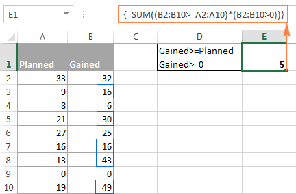
Remember to press Ctrl + Shift + Enter to enter the Excel array formula correctly.
The next couple of paragraphs are intended for those who like looking under the hood. If you are not interested in tech details, you can skip right to the next formula example.
For better understanding of this formula in particular and Excel array formulas in general, let's select the two expressions within the SUM function's parentheses in the formula bar, and press F9 to view the arrays behind the formula parts. If you want more information on how the F9 key works, please check out Evaluating portions of an array formula with F9.
So, what we have here is two arrays of Boolean values, where TRUE equates to 1 and FALSE equates to 0. Since we are using the AND array operator (*) in the formula, SUM will add up only those rows that have TRUE (1) in both arrays, as shown in the screenshot below:

Note. Not all Excel functions that support arrays can convert TRUE and FALSE into 1 and 0. In more complex array formulas, you might need to use a double dash (--), which is technically called the double unary operator, to convert non-numeric Boolean values to numbers.
Including a double dash in the above formula won't do any harm either, it will just keep you on the safe side: =SUM(--(B2:B10>=A2:A10) * (B2:B10>0))
And here is a more sophisticated Excel array formula example that absolutely requires the use of the double unary operator.
Example 2. Using several functions in Excel array formulas
Array formulas can work with several Excel functions at a time and perform multiple calculations within a single formula.
For example, if you have a table listing multiple product sales by several salesmen, and you want to know the maximum sale made by a given person for a given product, you can write an array formula based on the following pattern:
Assuming that the sales person names are in column A, product names are in column B and sales are in column C, the following formula returns the largest sale Mike has made for Apples:
=MAX(IF(($A$2:$A$9="mike") * ($B$2:$B$9="apples"), $C$2:$C$9,""))
Naturally, you can replace the names in the formula with cell references so that your users can simply type the names in certain cells without modifying your array formula:
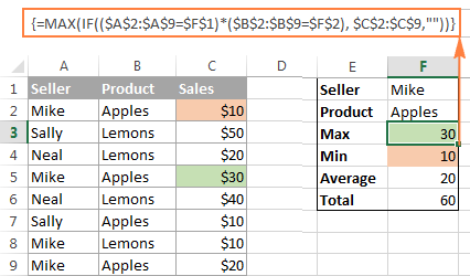
In the screenshot above, the following Excel array formulas are used (don't forget to press Ctrl + Shift + Enter to enter them correctly):
Maximum: =MAX(IF(($A$2:$A$9=$F$1) * ($B$2:$B$9=$F$2), $C$2:$C$9,""))
Minimum: =MIN(IF(($A$2:$A$9=$F$1) * ($B$2:$B$9=$F$2), $C$2:$C$9,""))
Average: =AVERAGE(IF(($A$2:$A$9=$F$1) * ($B$2:$B$9=$F$2), $C$2:$C$9,""))
Total: =SUM(IF(($A$2:$A$9=$F$1) * ($B$2:$B$9=$F$2), $C$2:$C$9,""))
Example 3. Array formula to count all characters in a range
This array formula example shows how you can count the number of characters, including spaces, in a range of cells.
The formula is as simple as this:
You use the LEN function to return the length of the text string in each individual cell, and then you use the SUM function to add up those numbers.
For example, the array formula =SUM(LEN(A1:A10)) calculates the total number of all chars with spaces in range A1:A10.
Example 4. Array formula to count specific character(s) in a range
If you want to know how many times a given character or a group of characters appears in a specified range of cells, an array formula with the LEN function can help again. In this case, the formula is a bit more complex:
And here is a practical example. Suppose, you have a list of orders where one cell may contain several order numbers separated by commas or any other delimiter. There are several order types and each has its own unique identifier - the first character in an order number.
Assuming that orders are in cells B2:B5 and the unique identifier in E1, the formula is as follows:
=SUM((LEN(B2:B5) - LEN(SUBSTITUTE(B2:B5, E1, ""))) / LEN(E1))
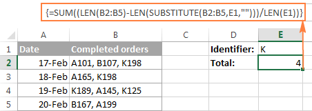
At the heart of this formula, the SUBSTITUTE function replaces all occurrences of the specified character with an empty string ("").
The substituted string is fed to the LEN function to get the string length without the character of interest ("K" in this example). And then, you subtract the length of the substituted string from the original string's length. The result of this operation is an array of character counts, one per cell, which you divide by the substring length. The operation of division is not strictly necessary when you count a single character like in this example. But if you are counting the occurrences of a specific substring in a range (e.g. orders beginning with "KM"), you do need to divide by the substring length, otherwise each character in the substring will be counted individually.
Finally, you use SUM to add up the individual counts.
Example 5. Sum values in every other or Nth row
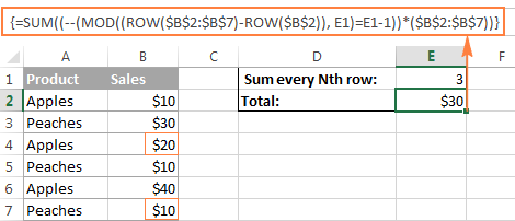
If you want to sum every other or every Nth row in a table, you will need the SUM and MOD functions combined in an array formula:
The MOD function returns the remainder rounded to the nearest integer after the number is divided by the divisor. We embed the ROW function into it to get the row's number, and then divide it by the Nth row (e.g. by 2 to sum every second cell) and check if the remainder is zero. If it is, then the cell is summed.
The double unary operator (--) is used to convert non-numeric Boolean values TRUE and FALSE returned by MOD into 1 and 0 for the SUM function to be able to add up the numbers.
For example, to count every other cell in range B2:B10, you use one of the following formulas:
Count even rows (2nd, 4th, etc.):
=SUM((--(MOD(ROW($B2:B10), 2)=0))*(B2:B10))
Count odd rows (1st, 3rd, etc.):
=SUM((--(MOD(ROW($B2:B10), 2)=1))*(B2:B10))
To get a universal formula that can sum values in any Nth rows that you specify and work correctly with any ranges regardless of their location in a worksheet, the formula has to be improved a little further:
=SUM((--(MOD((ROW($B$2:$B$7)-ROW($B$2)), E1)=E1-1))*($B$2:$B$7))
Where E1 is every N row you want to sum.
Example 6. Perform different calculations on numbers within different ranges
Here is a typical situation for many vendors - the unit price varies depending on the purchased quantity, and your goal is to write a formula that calculates the total price for any amount input in a specific cell.
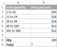
This task can be easily accomplished by using the following nested IF formula:
=B8*IF(B8>=101,B6, IF(B8>=50, B5, IF(B8>=20, B4, IF( B8>=11, B3, IF(B8>=1, B2, "")))))
However, this approach has a significant limitation. Because the formula references each price in cells B2 to B6 individually, you will have to update the formula as soon as your users change any of the existing ranges or add a new quantity range.
To make the formula more flexible, operate on arrays rather than individual cells. In this case, no matter how many values are changed, added or deleted, you will only have to update a single range reference in the formula.
=SUM(B8*(B2:B6) * (--(B8>=VALUE(LEFT(A2:A6,FIND(" ",A2:A6))))) * (--(B8<=VALUE(RIGHT(A2:A6,LEN(A2:A6) - FIND(" to ",A2:A6)-LEN(" to" ))))))
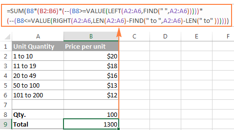
The detailed break down of this formula will probably require a separate article, so I will make just a quick overview of the logic. If you select individual parts of the formula in the formula bar and press F9, you will see that it boils down to evaluating the following 3 arrays (provided the quantity in B8 is 100 like in the screenshot above):
=SUM(B8*{20;18;16;13;12}*{1;1;1;1;0}*{0;0;0;1;1})
The first 5-element array is nothing else than the price numbers in cells B2:B6. And the last 2 arrays of 0's and 1's determine which price will be used in calculation. So, the main question is - where do these two arrays come from and what do they mean?
The formula includes 2 VALUE functions: (B8>=VALUE())*(B8<=VALUE())
The 1st function checks if the value in B8 is greater than or equal to the lower bound of each "unit quantity" range, and the 2nd one checks if B8 is less than or equal to the upper bound of each range (the combinations of LEFT, RIGHT, FIND and LEN functions are used to extract the upper and lower bound values). As a result, you get 0 if the condition is not met, and 1 if the condition is met.
Finally, the SUM function multiplies the quantity in B8 by each element of the price array (B2:B6) and by each elements of the 0's and 1's arrays. Since multiplying by 0 always gives 0, only one price is used in the final calculation - the element that has 1's in the last two arrays.
In this example, the quantity is multiplied by $13 that corresponds to "50 to 100" amount range. It is the 4th item of the price array (cell B5 in range B2:B6), and it is the only element that has 1's in the last two arrays.
For the formula to work correctly, be sure to check these two things:
- The quantities in A2:A6 should constitute a contiguous range such that no value is left out.
- All quantities in A2:A6 have to be entered in this specific pattern "X to Y" because it is hard-coded in the formula. If your quantities are entered in a different way, say "1 - 10", then replace " to" with " -" in the formula.
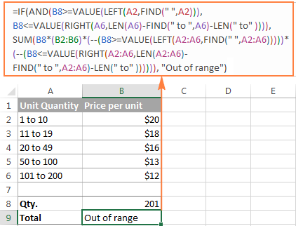
If you want to display an "Out of range" message when the quantity input in B8 is outside the amount range, include the following IF statement:
=IF(AND(B8>=VALUE(LEFT(A2,FIND(" ",A2))), B8<=VALUE(RIGHT(A6,LEN(A6) - FIND(" to ",A6)-LEN(" to" )))), SUM(…))
This complex If function does a very simple thing - checks if the value in B8 is greater than or equal to the lower bound in A2 and less than or equal to the upper bound in A6. In other words, it tests this condition: AND(B8>=1, B8<=200).
The complete formula goes as follows:
=IF(AND(B8>=VALUE(LEFT(A2,FIND(" ",A2))), B8<=VALUE(RIGHT(A6,LEN(A6)-FIND(" to ",A6)-LEN(" to" )))), SUM(B8*(B2:B6)*(--(B8>=VALUE(LEFT(A2:A6,FIND(" ",A2:A6)))))*(--(B8<=VALUE(RIGHT(A2:A6,LEN(A2:A6)-FIND(" to ",A2:A6)-LEN(" to" )))))), "Out of range")
Example 7. User-defined functions in Excel array formulas
This example is purposed for power users that have some knowledge of Excel VBA macros and user-defined functions.
You can utilize your own user-defined function in Excel array formulas, provided that a given function supports calculations in arrays.
For example, one of our Excel gurus wrote a function called GetCellColor that can get a color of all cells in a range, exactly as its name suggests. You can grab the function's code from this article - Sum and count colored cells in Excel.
And now, let's see how you can use the GetCellColor function in an array formula. Suppose you have a table with a color coded column and you want to sum the values that meet several conditions, including a cell's color. As an example, let's find the total of "green" and "yellow" sales made by Neal:
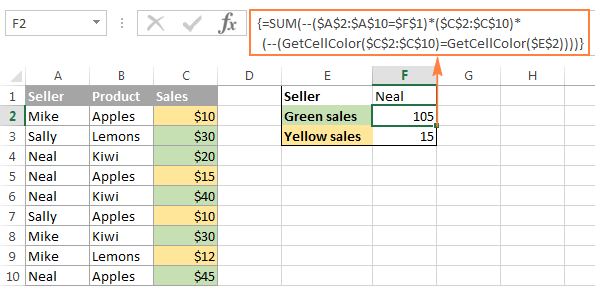
As demonstrated in the image above, we use the following Excel array formula:
=SUM(--($A$2:$A$10=$F$1) * ($C$2:$C$10) * (--(GetCellColor($C$2:$C$10)=GetCellColor($E$2))))
Where cell F1 is the sales person name and E2 is the color pattern.
The formula sums cells in the range C2:C10 if the following 2 conditions are met:
$A$2:$A$10=$F$1- checks if a cell in column A matches the seller name in F1, which is Neal in this example.GetCellColor($C$2:$C$10)=GetCellColor($E$2)- we use the custom user-defined function to get the color of cells C2 through C10, and check if it matches the color pattern in E2, green in this case.
Please pay attention that we use the double unary operator with both of the above expressions in order to convert the Boolean values TRUE and FALSE they return into 1's and 0's the SUM function can operate on. If both conditions are met, i.e. two 1's are returned, SUM adds up the sales amount from a corresponding cell in column C.
More Excel array formula examples
And here are a few more examples of Excel array formulas that might be helpful.
- Look up with multiple criteria - a powerful INDEX / MATCH function that can look up by values in 2 different columns.
- Get all duplicate values in the lookup range - how to get all instances of the lookup value.
- Case-sensitive lookup for all data types - self-explanatory : )
- Array LOOKUP and SUM - how to look up in an array and sum all matching values.
- Excel SUM function in array formulas - a few examples that demonstrate the uses of SUM in array formulas.
- Excel TRANSPOSE formula examples - how to convert rows to columns in Excel.
- Sum the largest or smallest numbers in a range - how to sum a variable number of largest / smallest values in the range.
Excel array formulas - limitations and alternatives
Array formulas are by far one of the most powerful features in Excel, but not all-powerful. Here are the most critical limitations of arrays in Excel.
1. Large arrays may slow down Excel
Though Microsoft Excel does not impose any limit on the size of arrays you use in your worksheets, you are limited by memory available on your computer because recalculating formulas with large arrays is time consuming. So, in theory, you can create huge arrays consisting of hundreds or thousands of elements, in practice this is not recommended because they can drastically slow your workbooks.
2. Entire column arrays are not allowed
You are not allowed to create an array that includes a whole column or several columns for an obvious reason explained above. Array formulas in Excel are very resource-hungry and Microsoft is taking preventive measures against Excel's freezing.
3. Limit to array formulas referring to another sheet
In Excel 2003 and earlier versions, a given worksheet could contain a maximum of 65,472 array formulas referring to another sheet. In modern versions of Excel 2013, 2010 and 2007, cross-worksheet array formulas are limited by available memory only.
4. Debugging array formulas
If your array formula returns an incorrect result, make sure you pressed Ctrl + Shift + Enter when entering it. If you did, select parts of the formula and press the F9 key to evaluate and debug them.
5. Alternatives to array formulas.
If you find Excel array formulas too complex and confusing, you can use one of Excel functions that can naturally process arrays of data (without pressing Ctrl + Shift + Enter). A good example is the SUMPRODUCT function that multiplies values in the specified arrays and returns the sum of those products. Another example is Excel INDEX function with an empty value or 0 in the row_num or col_num argument to return an array of values from the entire column or row, respectively.
If you want to download the Excel array formula examples discussed in this tutorial to reverse-engineer them for better understanding, you are most welcome to download formula examples. This is an .xlsm file since example 6 includes a custom VBA function, so you will have to click the Enable Content button after downloading to allow the macro to run.
That's all for today, thank you for reading!
 by
by
28 comments
Hi,
Very good perspective on Array Formulas ...
Can an Array Formula replicate the "Step" feature offered by the very recent Sequence function ?
The objective for the Array Formula is to generate {1,4,7,10,13} (working with Excel 2016)
Thanks for your insight
Hello!
As an alternative to the SEQUENCE function, try this formula:
=1+(ROW(A1:A5)-1)*3
Hope this is what you need.
Hi,
I'm trying to make a list where the value increases based on some other results or not. It references the cell above each value, and the array spill in 365 mistakenly claims that there is a circular reference. How to fix?
C5 =0
C6 =if(C5:C100>5,0,C5:c100+1)
The actual boolean is a bit more complicated, and many thousands of rows, but it shows the problem.
This really seems to limit the usability of autospill if it cannot be fixed somehow.
Thanks, looking forward to any insights
Hi!
The formula in cell C6 refers to itself because C6 is in the range C5:C100.
Read more in this article: Circular reference in Excel: how to find, enable, use, or remove.
= switch(B3, 1, "JANUARY", 2, "FEBRUARY", 3, "MARCH", 4, "APRIL", 5, "MAY", 6, "JUNE", 7, "JULY", 8, "AUGUST", 9,"SEPTEMBER", 10,"OCTOBER", 11, "NOVEMBER ", 12, "DECEMBER")
When I run this function , error type "#name?" . I am using EXCEL 16 . will you kindly debug?
Hi!
This function is available if you have Office 2019 or Office365
asd | 0.01 | 0.02 | -0.03
ase| 0.02 | 0.03 | -0.03
asf | 0.03 | 0.04 | -0.10
asg | 0.04 | 0.05 | -0.11
ash | 0.05 | 0.06 | -0.11
For example A is the order id, others are price, if i wan get the order id after SUM up B,C,D < 0 how can i do that? For this one, i wan the result is asf and asg. Please help me with formula
Hello!
Please try the following array formula:
{=IFERROR(INDEX($A$3:$A$12, SMALL(IF(($E$3:$E$12+$D$3:$D$12+$C$3:$C$12)<0, ROW($A$3:$A$12)- MIN(ROW($A$3:$A$12))+1,""), ROW()-2)),"")}
Hope this is what you need.
In the above tutorial you use a User-Defined function called "GetCellColor". I assume that since it is Alexander Frolov design we can NOT utilize it within the tutorial review. It's a non-function on my laptop, Correct? If so, why not advise within the tutorial? In an attempt to understand your tutorial I recreate each and very Example to ensure I understand the section. I can NOT get Example 7 to work. It comes back with an error message "NAME".
thoughts?
Thanks
Hello Gregg,
Thank you for your comment.
To be able to use this function, you need to add its VBA code to your Excel. The code and the detailed instructions are provided in a separate article: How to count and sum cells by color in Excel.
Because the focus of this tutorial is on array formulas, we did not replicate the code here. Instead, I included the above link in the corresponding example.
Hi!!! Please (First of all, sorry my english!) So! I need a array formula to return another array with the Match Maximum Value in each row. Something like this:
0 1 3
1 5 4
9 8 3
return: {3,5,9}
Just it!! Tks a lot!
I to do that with just one row! But a need a array formula to do it with an array...
example:
A B C
ROW-1 0 1 5
=match(max(A1:C1),A1:C1,0) = 3
IF IN THE PARTICULAR COLUMN THE CELL CONTAIN A,B AND C ALPHABET, HOW WE WILL SET THE FORMULA FOR COUNTING ONLY A & B TOGETHER.
EXAMPLE:
A
A
B
C
B
COUNTING SHOULD BE 4.
PLEASE ADVICE
Suppose cell address of A is A1 & last B has address A5. Then the formula will be-
=countif(A1:A5,"A")+countif(A1:A5,"B")
I think this will serve the purpose.
Hi there!!!
Something, that I think is curious, is why, in your fourth example, you put "/ LEN(E1)" in your formula. According to me, you didn't need it: You can obtain the same result without it. But, any way, if you have time and you like, would you like to explain me? To me it would be something very illustrative.
Take care, and thanks for your knowledge.
Hi Sergio,
Dividing by LEN(E1) is not needed when you count a single character like in the example you referred to. In situations when you want to count the occurrences of a specific substring in a range (i.e. a sequence of 2 or more characters), you need to divide by the substring length, otherwise each character in the substring will be counted individually (for example if you have entries like "cat-1", "cat-2", "dog-1, "dog-2", etc. and you want to get the total number of "cat" entries).
hi there,
I am trying to make a barcode scanner excel sheet. suppose in one coloum A, i have barcode numbers like 123456789, 987654321 etc and in colum B i have their names like product X, product Y etc. i want if i scan a barcode in column C and if it is present in the list A, it must be display its product name name from column B and if not present it must display any other message. can anyone help me out with a formula ?
thanks
If you want just to verify if Cx=Ax, then is really simple.
=IF(C2=A2,B2,"")
Copy formula in all column C cells (your range, not full column C).
hello,
your site is great and i found it very useful.
would you have an examples of calculations such as this: =SUMIF([Timeline],"<="&[@Timeline],[Weighted Forecast]).
Thanks a lot,
Ziv
Hello, Ziv,
For us to be able to assist you better, please describe your task in more detail and give more examples.
Dear, I have amount in cell A Rs:642. I need formula that show in next cell (B) only that amount multiply by 25.
For example: A B C A B C
642 625 17 366 350 16
=sum(A1*25) this will do it for you.
Hi Svetlana,
Your article, methinks, is the best to start learning Array Formulas.
Great job!
Shall I expect an article that describes
*Add-ins,
*Simplifying big formulas into small etc.?
Hi Prasad,
Thank you so much for your kind feedback and the idea. I will give it a thought :)
Very informative article which I have benefited greatly from. Thank you for sharing.
Nova Scotia, Canada
Thank you, Rick!
this formula worked for me =SUM((LEN(C5:AF5)-LEN(SUBSTITUTE(C5:AF5, AH3,"")))/LEN(AH3))
but when I Drag this formula for the below column.... this formula doesn't apply..... why is that..... this is exactly what I was looking for but at dragging the formula from top to bottom the formula changes and from C the formula goes to D and from AF5 it goes to AF6
Example :
Top Column = =SUM((LEN(C4:AF4)-LEN(SUBSTITUTE(C4:AF4, AH3,"")))/LEN(AH3))
when I drag formula from top to bottom of the spreadsheet
the formula changes to
=SUM((LEN(C5:AF5)-LEN(SUBSTITUTE(C5:AF5, AH4,"")))/LEN(AH4))
Hi Adrian,
Just fix the cell references that shouldn't be changed with the $ sign.
For example, if you need to fix the range C4:AF4, then write LEN($C$4:$AF$4)...
You can learn more about absolute (with $) and relative (without $) cell references in this tutorial:
https://www.ablebits.com/office-addins-blog/relative-absolute-reference-excel/