In this article, you will learn various ways to concatenate text strings, numbers and dates in Excel using the CONCATENATE function and "&" operator. We will also discuss formulas to combine individual cells, columns and ranges.
In your Excel workbooks, the data is not always structured according to your needs. Often you may want to split the content of one cell into individual cells or do the opposite - combine data from two or more columns into a single column. Common examples are joining names and address parts, combining text with a formula-driven value, displaying dates and times in the desired format, to name a few.
In this tutorial, we are going to explore various techniques of Excel string concatenation, so you can choose the method best suited for your worksheets.
What is "concatenate" in Excel?
In essence, there are two ways to combine data in Excel spreadsheets:
- Merging cells
- Concatenating cells' values
When you merge cells, you "physically" join two or more cells into a single cell. As a result, you have one larger cell that is displayed across multiple rows and/or columns.
When you concatenate cells in Excel, you combine only the contents of those cells. In other words, concatenation in Excel is the process of joining two or more values together. This method is often used to combine a few pieces of text that reside in different cells (technically, these are called text strings or simply strings) or insert a formula-calculated value in the middle of some text.
The following screenshot demonstrates the difference between these two methods:

Merging cells in Excel is the subject of a separate article, and in this tutorial, we'll discuss the two main ways to concatenate strings in Excel - by using the CONCATENATE function and the concatenation operator (&).
Excel CONCATENATE function
The CONCATENATE function in Excel is used to join different pieces of text together or combine values from several cells into one cell.
The syntax of Excel CONCATENATE is as follows:
Where text is a text string, cell reference or formula-driven value.
The CONCATENATE function is supported in all versions of Excel 365 - 2007.
For example, to concatenate the values of B6 and C6 with a comma, the formula is:
=CONCATENATE(B6, ",", C6)
More examples are shown in the image below:
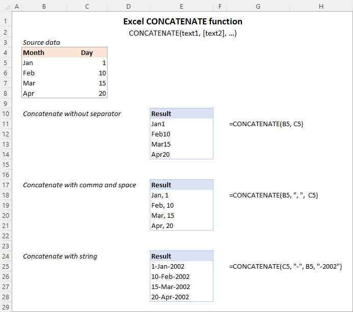
Note. In Excel 365 - Excel 2019, the CONCAT function is also available, which is a modern successor of CONCATENATE with exactly the same syntax. Although the CONCATENATE function is kept for backward compatibility, Microsoft does not give any promises that it will be supported in future versions of Excel.
Using CONCATENATE in Excel - things to remember
To ensure that your CONCATENATE formulas always deliver the correct results, remember the following simple rules:
- Excel CONCATENATE function requires at least one "text" argument to work.
- In one formula, you can concatenate up to 255 strings, a total of 8,192 characters.
- The result of the CONCATENATE function is always a text string, even when all of the source values are numbers.
- Unlike the CONCAT function, Excel CONCATENATE does not recognize arrays. Each cell reference must be listed separately. For example, you should use CONCATENATE(A1, A2, A3) and not CONCATENATE(A1:A3).
- If any of the arguments is invalid, the CONCATENATE function returns a #VALUE! error.
"&" operator to concatenate strings in Excel
In Microsoft Excel, the ampersand sign (&) is another way to concatenate cells. This method comes in very handy in many scenarios since typing an ampersand is much faster than typing the word "concatenate" :)
For example, to concatenate two cell values with a space in-between, the formula is:
=A2&" "&B2
How to concatenate in Excel - formula examples
Below you will find a few examples of using the CONCATENATE function in Excel.
Concatenate two or more cells without separator
To combine the values of two cells into one, you use the concatenation formula in its simplest form:
=CONCATENATE(A2, B2)
Or
=A2&B2
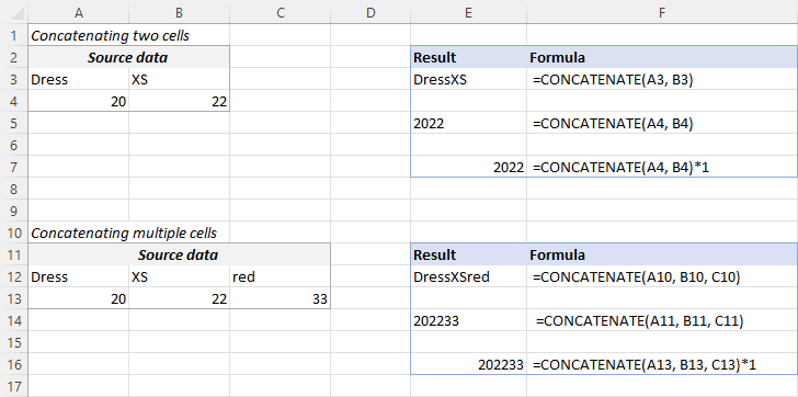
Please note that the values will be knit together without any delimiter like in the screenshot below.
To concatenate multiple cells, you need to supply each cell reference individually, even if you are combining contiguous cells. For example:
=CONCATENATE(A2, B2, C2)
Or
=A2&B2&C2
The formulas work for both text and numbers. In case of numbers, please keep in mind that the result is a text string. To convert it to number, just multiply CONCATENATE's output by 1 or add 0 to it. For instance:
=CONCATENATE(A2, B2)*1
Tip. In Excel 2019 and higher, you can use the CONCAT function to quickly concatenate multiple cells using one or more range references.
Concatenate cells with a space, comma or other delimiter
In your worksheets, you may often need to join values in a way that includes commas, spaces, various punctuation marks or other characters such as a hyphen or slash. To do this, simply put the desired character in your concatenation formula. Remember to enclose that character in quotation marks, as demonstrated in the following examples.
Concatenating two cells with a space:
=CONCATENATE(A2, " ", B2)
or
=A2 & " " & B2
Concatenating two cells with a comma:
=CONCATENATE(A2, ", ", B2)
or
=A2 & ", " & B2
Concatenating two cells with a hyphen:
=CONCATENATE(A2, "-", B2)
or
=A2 & "-" & B2
The following screenshot demonstrates how the results may look like:

Tip. In Excel 2019 and higher, you can use the TEXTJOIN function to merge strings from multiple cells with any delimiter that you specify.
Concatenating text string and cell value
There is no reason for the Excel CONCATENATE function to be limited to only joining cells' values. You can also use it to combine text strings to make the result more meaningful. For example:
=CONCATENATE(A2, " ", B2, " completed")
The above formula informs the user that a certain project is completed, as in row 2 in the screenshot below. Please notice that we add a space before the word " completed" to separate the concatenated text strings. A space (" ") is also inserted between the combined values, so that the result displays as "Project 1" rather than "Project1".
With the concatenation operator, the formula can be written this way:
=A2 & " " & B2 & " completed"
In the same manner, you can add a text string in the beginning or in the middle of your concatenation formula. For example:
=CONCATENATE("See ", A2, " ", B2)
="See " & A2 & " " & B2

Join text string and another formula
To make the result returned by some formula more understandable for your users, you can concatenate it with a text string that explains what the value actually is.
For example, you can use the following formula to return the current date in the desired format and specify what kind of date that is:
=CONCATENATE("Today is ",TEXT(TODAY(), "mmmm d, yyyy"))
="Today is " & TEXT(TODAY(), "dd-mmm-yy")

Tip. If you would like to delete the source data without affecting the resulting text strings, use the "Paste special - values only" option to convert formulas to their values.
Concatenate text strings with line breaks
Most often, you would separate the resulting text strings with punctuation marks and spaces, as shown in the previous example. In some cases, however, there may be a need to separate the values with a line break, or carriage return. A common example is merging mailing addresses from data in separate columns.
A problem is that you cannot simply type a line break in the formula like a usual character. Instead, you use the CHAR function to supply the corresponding ASCII code to the concatenation formula:
- On Windows, use CHAR(10) where 10 is the character code for Line feed.
- On Mac, use CHAR(13) where 13 is the character code for Carriage return.
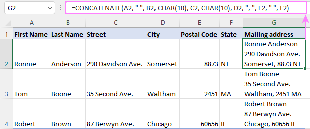
In this example, we have the address pieces in columns A through F, and we are putting them together in column G by using the concatenation operator "&". The merged values are separated with a comma (", "), space (" ") and a line break CHAR(10):
=A2 & " " & B2 & CHAR(10) & C2 & CHAR(10) & D2 & ", " & E2 & " " & F2
The CONCATENATE function would take this shape:
=CONCATENATE(A2, " ", B2, CHAR(10), C2, CHAR(10), D2, ", ", E2, " ", F2)
Either way, the result is a 3-line text string:
In the same manner, you can separate final strings with other characters such as:
- Double quotes (") - CHAR(34)
- Forward slash (/) - CHAR(47)
- Asterisk (*) - CHAR (42)
- The full list of ASCII codes is available here.
How to concatenate columns in Excel
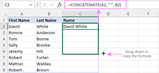
To join two or more columns, just enter your concatenation formula in the first cell, and then copy it down to other cells by dragging the fill handle (the small square that appears in the lower right hand corner of the selected cell).
For example, to combine two columns (column A and B) delimiting the values with a space, the formula in C2 copied down is:
=CONCATENATE(A2, " ", B2)
Or
= A2 & " " & B2
For more information, please see How to merge two columns in Excel without losing data.
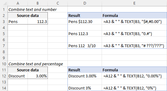
Combine text and numbers keeping formatting
When concatenating a text string with a number, percentage or date, you may want to keep the original formatting of a numeric value or display it in a different way. This can be done by supplying the format code inside the TEXT function, which you embed in a concatenation formula.
In the beginning of this tutorial, we have already discussed a formula that concatenates text and date.
And here are a few more formula examples that combine text and number:
Number with 2 decimal places and the $ sign:
=A2 & " " & TEXT(B2, "$#,#0.00")
Number without insignificant zeros and the $ sign:
=A2 & " " & TEXT(B2, "0.#")
Fractional number:
=A2 & " " & TEXT(B2, "# ?/???")
To concatenate text and percentage, the formulas are:
Percent with two decimal places:
=A12 & " " & TEXT(B12, "0.00%")
Rounded whole percent:
=A12 & " " & TEXT(B12, "0%")
How to concatenate a range of cells in Excel
Combining values from multiple cells might take some effort because the Excel CONCATENATE function does not accept arrays.
To concatenate several cells, say A1 to A4, you need to use one of the following formulas:
=CONCATENATE(A1, A2, A3, A4)
or
=A1 & A2 & A3 & A4
When combining a fairly small group of cells, it's no big deal to type all the references. A large range would be tedious to supply, typing each individual reference manually. Below you will find 3 methods of quick range concatenation in Excel.
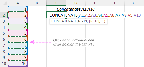
Method 1. Press CTRL to select multiple cells
To quickly select several cells, you can press and hold the Ctrl key while clicking on each cell you want to include in the formula. Here are the detailed steps:
- Select a cell where you want to enter the formula.
- Type =CONCATENATE( in that cell or in the formula bar.
- Press and hold Ctrl and click on each cell you want to concatenate.
- Release the Ctrl button, type the closing parenthesis, and press Enter.
Method 2. Use TRANSPOSE function to get all cell values
When a range consists of tens or hundreds of cells, the previous method may not be fast enough as it requires clicking on each cell. In this case, you can use the TRANSPOSE function to return an array of values, and then merge them together in one fell swoop.
- In the cell where you want the result to appear, enter the TRANSPOSE formula, for example:
=TRANSPOSE(A1:A10)
- In the formula bar, press F9 to replace the formula with calculated values. As a result, you will have an array of values to be concatenated.
- Delete the curly braces surrounding the array.

- Type =CONCATENATE( before the first value, then type the closing parenthesis after the last value, and press Enter.

Note. The result of this formula is static as it concatenates the values, not cell references. If the source data changes, you will have to repeat the process.
Method 3. Use the CONCAT function
In Excel 365 and Excel 2021, this simple formula will concatenate a range of cells in a blink:
=CONCAT(A1:A10)
Method 4. Use the Merge Cells add-in
A quick and formula-free way to concatenate any range in Excel is to use the Merge Cells add-in with the "Merge all areas in selection" option turned off, as demonstrated in Combining values of several cells into one cell.
Excel "&" operator vs. CONCATENATE function
Many users wonder which is a more efficient way to join strings in Excel - CONCATENATE function or "&" operator.
The only real difference is the 255 strings limit of the CONCATENATE function and no such limitation when using the ampersand. Other than that, there is no difference between these two methods, nor is there any speed difference between the CONCATENATE and "&" formulas.
And since 255 is a really big number and you will hardly ever need to combine that many strings in real work, the difference boils down to comfort and ease of use. Some users find CONCATENATE formulas easier to read, I personally prefer using the "&" method. So, simply stick with the technique you feel more comfortable with.
Opposite of CONCATENATE in Excel (splitting cells)
The opposite of concatenate in Excel is splitting the contents of one cell into multiple cells. This can be done in a few different ways:
- Text to Columns feature
- Flash Fill option in Excel 2013 and higher
- TEXTSPLIT function in Excel 365
- Custom formulas to split cells (MID, RIGHT, LEFT, etc.)
You can also find useful information in this article: How to unmerge cells in Excel.
Concatenate in Excel with Merge Cells add-in
With the Merge Cells add-in included in Ultimate Suite for Excel, you can efficiently do both:
- Merge several cells into one without losing data.
- Concatenate the values of several cells into a single cell and separate them with any delimiter of your choosing.
The Merge Cells tool works with all Excel versions from 2016 to 365 and can combine all data types including text strings, numbers, dates and special symbols. Its two key advantages are simplicity and speed - any concatenation is done in a couple of clicks.
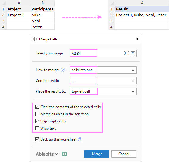
Combine values of several cells into one cell
To combine the contents of several cells, you select the range to concatenate and configure the following settings:
- Under What to merge, select Cells into one.
- Under Combine with, type the delimiter (a comma and a space in our case).
- Choose where you want to place the result.
- Most importantly, uncheck the Merge all areas in the selection box. It is this option that controls whether the cells are merged or their values are concatenated.
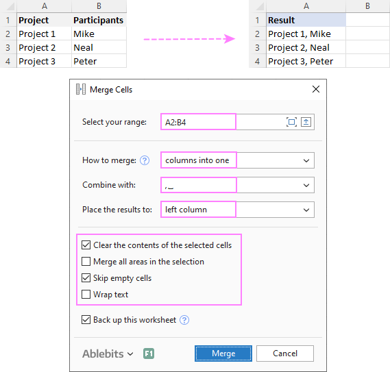
Combine columns row-by-row
To concatenate two or more columns, you configure the Merge Cells' settings in a similar way but choose to merge columns into one and place the results in the left column.
Join rows column-by-column
To combine data in each individual row, column-by-column, you choose:
- Merge rows into one.
- Use a line break for the delimiter.
- Place the results in the top row.
The result may look similar to this:
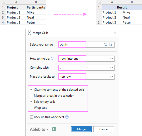
To check how the Merge Cells add-in will cope with your data sets, you are welcome to download a fully functional trial version of our Ultimate Suite for Excel below.
That's how to concatenate in Excel. I thank you for reading and hope to see you on our blog next week!
Available downloads
Concatenation formula examples (.xlsx file)
Ultimate Suite 14-day trial version (.exe file)
 by
by
267 comments
I have an XLOOKUP(A12, TeamA1Week, TeamA1Rink), which works well. However I want to extend it, so that the 'A1' is replaced by the contents of K4, which could be A1 to A4, B1 to B5, C1 to C6 etc.
So how do I replace the 'A1' in 'TeamA1Week', with the contents of K4, have tried Concatenate, but no luck.
Regards
Tim
Hello Tim!
If I understand your formula correctly, TeamA1Week is a named range. If you want to use a different name in the formula, that name must exist in your workbook.
Use the INDIRECT function to build the range name as text and then reference it:
=XLOOKUP(A12, INDIRECT("Team" & K4 & "Week"), TeamA1Rink)
Read more: INDIRECT with named ranges
Hi, thanks very much exactly what I wanted.
Merge 0.5 and "kg" ... output is 0.5kg but I want 1/2kg what I do...any formula have give me bro...for my catering business grocery Excel sheet
Hi! Use the custom number format as recommended in these instructions: Turn decimal numbers into fractions. Use the TEXT function to write a number in this format as text and combine it with a text string:
=TEXT(I12,"1/2")&"kg"
Hello,
I am looking for a way to remove blank lines in a cell that has multiple lines.
For instance, a description field that has
"I am line 1"
"I am line 3"
How can I remove the blank line between lines 1 & 3 for thousands of records in the spreadsheet? I want it to look like this;
"I am line 1"
"I am line 3"
Thanx!!!!
Hi! If I understand your task correctly, look for the example formulas here: How to delete line breaks and nonprinting characters.
Is it possible for this scenario?
For explanation purposes,:
(B) as bold start, (/B) end
(i) as italic, (/i) end
Plotted in Excel:
A1= Maria; A2=has; A3=Apples
The result needed in one cell is to be:
Maria has Apples as (B) Maria (/B) (i) has (/i) (B)(i) Apples (/i)(/B)
what formula do I need to come up to that function?
I have been researching for a formula for a week now, hope you understood my scenario
Hi! Excel formula cannot copy or set the cell format. Therefore, your scenario is only possible with VBA code. Or you can manually set the format of specific words within a cell.
Thanks for the response!
Any idea for a VBA code for these? Thank you.
I am working on a sheet that has info like this:
Date UDB01 UDB02
W - 11/1/2023 67.20% 34.50%
T - 11/2/2023 67.20% 34.50%
I have individual charts for each showing trending for database space. I am trying to concatenate the chart title the first cell in the column and the last cell which is a percentage. Everyday a new last cell gets added to the columns. I have followed your page on concatenate to be able to join the cells but it always converts the percentage to a decimal and I cant figure out if there is a way to have it join them based on the new next final percentage cell. Is this possible? Thanks ahead of time!!!!!!
Example chart tile would be B1&" - "&B3 resulting in: UDB01 - 67.20%
Hi! If you want to combine text and number in percentage format, use the TEXT function. For example:
=A1&TEXT(B1,"##.##%")
Hello! I have large data in row1 through several columns (A1:BLI1) and I want it all in column A. Can this be done?
Hi! Try to use the recommendations described in this article: Merge and combine cells in Excel without losing data.
My data table is
A, Hello
B, Hi
C, John
D, Joe,
I need a formula wherein if a cell contains the string "AC", result is Hello John, etc..
Please help
Hi! To use the CONCATENATE function by condition, use the IF function. The formula might look like this:
=IF(D1="AC",CONCATENATE(A1," ",A3))
I hope it’ll be helpful. If this is not what you wanted, please describe the problem in more detail.
I will have a long data table but let’s just limit it to from A1:B4
Cells A1:A4 values are a, b, c, d
Cells B1:4 values are Hello, Hi, john, joe.
D1 will be a variable that I will encode a value in (e.g., “ab”, “abc”, “ac”, “abcd”, etc.)
I will need a formula that can recognize that if D1 has a character “a” it will point to B1 and Concatenate this with other characters in the string in D1 (e.g., “b” to B2, “c” to B3, etc.). As such, it is supposed to variably concatenate 1-4 cells. There are no repeating characters in D1.
Hi! Split the text in D1 by character using the MID function. Find the values in column B that match the character in column A using INDEX MATCH function. Merge these values into a text string using the TEXTJOIN function.
=TEXTJOIN(", ",TRUE,IFERROR(INDEX(B1:B4,MATCH(MID(D1,ROW(A1:A4),1),A1:A4,0)),""))
Damn, you're great! THANKS!!!
I'm working on a concatenate formula for a spreadsheet that contains several columns of data that are used to create a filename. I've finessed everything except one final step and I'm hitting a wall with that one.
This is an example of the data I'm using:
Name Last 4 Type Order # Order Start Order End Agency
Smith, J 1234 POC 456123 1/1/2023 3/1/2023 HHC Agency
Smith, J 1234 PO 789456 1/1/2023 ~ HHC Agency
This is my formula:
=CONCATENATE(A3," ",TEXT(B3,"0000"),", ",C3,", ",TEXT(E3,"mmddyy"),"-",TEXT(F3,"mmddyy"),", ",D3,", ",G3)
It returns the desired filename for the first example (Smith, J 1234, POC, 010123-030123, 456123, HHC Agency) however for the 2nd example, I'm trying to figure out if I can tell it to NOT include the ~ in the final result.
This is what I get:
Smith, J 1234, PO, 010123-~, 789456, HHC Agency
But this is what I want:
Smith, J 1234, PO, 010123, 789456, HHC Agency
I'm fully accepting that this may be asking more of excel than it is able to give and, honestly, it's not a big deal, I've just gotten in very deep making this pretty so it's more a matter of personal success than necessity.
Thanks!
Hi! If I understand your task correctly, this article may be helpful: How to remove characters/text from string in Excel. Replace unwanted characters with a blank.
=SUBSTITUTE(A2,"-~","")
Two cell data merge , one column data is bold letters and another column data normal letter in required in one cell...It is possible????
When merging data from different columns, their format is not preserved.
I have a large data file that I am inputing manually at work.but am trying to create an easy short cut where if I input a value in a cell, other 2 corresponding or connecting cells must display their own value or information. For example;
Cell A1 input is FGOOO5 which is an item code for a product (in other words it's static of fixed).
What I want to do is create a system where whenever I type in FGOOO5 in cell A1, other corresponding cell or cells will display information such as its product name, and price automatically.
I need help please.
Hi! To find values according to the product code, try using the INDEX MATCH function. For detailed instructions and examples, read here: Excel INDEX MATCH vs. VLOOKUP - formula examples. You can also use the VLOOKUP function or the XLOOKUP function.
Thank you so much sir.
Hello - I'm trying to see if the following is a possible function in excel:
Cell: Shirt
Cell: Size
Cell: QTY
Cell: Price
Cell: Total
I'm trying to create a combination where a drop down of an item that has a price to it can automatically update the total by after selecting item, size and QTY. I hope that makes sense. Thank you!
Hi! If you want to dynamically create a list of prices for the chosen criteria, use these instructions: Create drop down list in Excel: static, dynamic, editable, searchable.
For example, write this formula in cell E3:
=FILTER(D3:D20,(A3:A20=K1)*(B3:B20=K2)*C3:C20=K3)
K1,K2.K3 - Shirt, Size,Qty
Then create dropdown list with source: =$E$3#
Hope this is what you need.
Please suggest me formula how to merge all Name data in one cell i have more 300 name
Rahul1
Samir2
Suresh3
Amit4
Rahul5
Samir6
Suresh7
Amit8
Rahul9
Samir10
Hi! To combine the values of a range of cells into one cell, you can use the CONCAT function, TEXTJOIN function, Merge Cells add-in for Excel.
I have two cells - cell 1 value i s abc while cell2 value is def (but e is formatted with strike out). how can I concatenate two cells by keeping format of Cell2 i.e. letter e with strike out formatting
Hi!
Unfortunately, the format can only be set for the whole cell, not for a single character.
It Should be possible to do with some macro, I guess
goodday, please assist me i have one cell with name and last name but with a space in between. How do i remove the space between .
Lucky Moo in one cell needs to be LuckyMoo in one cell.
Hello!
To remove a space, use the SUBSTITUTE function as described in this instruction: How to remove all spaces in Excel.
This should solve your task.
Thanks very much Alex, it worked.
A B OUTPUT
SAMADARSHI 123456 SAM123456XY
I NEED THIS TYPE OF OUTPUT CAN YOU SUGGEST FORMULA FOR THIS
Hi!
I hope you have studied the recommendations in the tutorial above and my answer to your previous question.
To extract the first 3 characters, use the substring functions MID or LEFT.
=MID(A1,1,3)&B1&"XY"
=LEFT(A1,3)&B1&"XY"
i Want Suggention multiple columns data combine one cell
Hi!
I recommend reading this guide: Merge and combine cells in Excel without losing data.
I hope it’ll be helpful.
I'm trying to concatenate two cells, if either cell has an #N/A in it I need the "#N/A" to appear as such in the concatenation, not the entire value of the field to return "#N/A."
Ex:
654321 #N/A
#N/A 123456
When concatenated I need these to read as such, "654321#N/A" and "#N/A123456"
Thank you.
Hello!
To handle the #N/A! error use the ISNA function. Replace the error with text and concatenate the cell values.
=IF(ISNA(A2),"#N/A",A2)&IF(ISNA(B2),"#N/A",B2)
I hope this will help.
Thank you so much!! I was sooooo close!!! :) That was just too "easy"!
Hello, is there code to format the color of individual strings when you splice them together with &? For example, the code below shows:
="Given the current inputs, there are enough supplies for "&'Inv 2/25/22'!O2&" days."
Could I add a command in this formula to change the color of what results from 'Inv 2/25/22'!O2, or even just make it bold?
Thank you!
Hello!
You can change the format of an entire cell either manually or using conditional formatting. You cannot change the format of part of a cell using a formula.
Hi
I'm having two values in two cells. I want to combine into single cell
Condition: one cell value must be same and second cell value must be in bracket and red colour. Is it possible?
7828.49(1589)
2846.35(1648)
Hello!
You cannot format a part of a cell in excel, for example, highlight it with a color. Only the entire cell can be formatted.
I concatenated a series of strings, I want it should act as a formula not text.
EX:- There is cell Value contains if statement and changes with the conditions provided, It is Showing value "L5"(it changes with conditions) in cell "e17", now I use concatenate formula "=concatenate("=",e17)" and I will get value "=L5" but I want that this "=L5" behave as a formula and show me the Value of the cell "L5".
Hello!
You can convert text to a formula using a VBA macro. Native Excel formulas won't do this.