When writing an Excel formula, $ in cell references confuses many users. But the explanation is very simple. The dollar sign in an Excel cell reference serves just one purpose - it tells Excel whether to change or not to change the reference when the formula is copied to other cells. And this short tutorial provides full details about this great feature.
The importance of Excel cell reference can hardly be overstated. Get the insight into the difference between absolute, relative and mixed references, and you are halfway to mastering the power and versatility of Excel formulas and functions.
All of you have probably seen the dollar sign ($) in Excel formulas and wondered what's that all about. Indeed, you can reference one and the same cell in four different ways, for example A1, $A$1, $A1, and A$1.
The dollar sign in an Excel cell reference affects just one thing - it instructs Excel how to treat the reference when the formula is moved or copied to other cells. In a nutshell, using the $ sign before the row and column coordinates makes an absolute cell reference that won't change. Without the $ sign, the reference is relative and it will change.
If you are writing a formula for a single cell, you can go with any reference type and get the formula right anyway. But if you intend to copy your formula to other cells, choosing the appropriate cell reference type is crucial. If you feel lucky, you can toss a coin :) If you want to be serious, then invest a few minutes in learning the ins-and-outs of absolute and relative cell references in Excel, and when to use which one.
What is an Excel cell reference?
To put it simply, a cell reference in Excel is a cell address. It tells Microsoft Excel where to look for the value you want to use in the formula.
For example, if you enter a simple formula =A1 in cell C1, Excel will pull a value from cell A1 into C1:

As already mentioned, as long as you write a formula for a single cell, you are free to use any reference type, with or without the dollar sign ($), the result will be the same:

But if you want to move or copy the formula across the worksheet, it's very important that you choose the right reference type for the formula to get copied correctly to other cells. The following sections provide the detailed explanation and formula examples for each cell reference type.
Note. Apart from the A1 reference style, where columns are defined by letters and rows by numbers, there also exist the R1C1 reference style where both rows and columns are identified by numbers (R1C1 designates row 1, column 1).
Because A1 is the default reference style in Excel and it is used most of the time, we will discuss only the A1 type references in this tutorial. If someone is currently using the R1C1 style, you can turn it off by clicking File > Options > Formulas, and then unchecking the R1C1 reference style box.
Excel relative cell reference (without $ sign)
A relative reference in Excel is a cell address without the $ sign in the row and column coordinates, like A1.
When a formula with relative cell references in copied to another cell, the reference changes based on a relative position of rows and columns. By default, all references in Excel are relative. The following example shows how relative references work.
Supposing you have the following formula in cell B1:
=A1*10
If you copy this formula to another row in the same column, say to cell B2, the formula will adjust for row 2 (A2*10) because Excel assumes you want to multiply a value in each row of column A by 10.

If you copy the formula with a relative cell reference to another column in the same row, Excel will change the column reference accordingly:

And if you copy or move an Excel formula with a relative cell reference to another row and another column, both column and row references will change:

As you see, using relative cell references in Excel formulas is a very convenient way to perform the same calculations across the entire worksheet. To better illustrate this, let's discuss a real-life example.
Using relative reference is Excel - formula example
Supposing you have a column of USD prices (column B) in your worksheet, and you want to convert them to EUR. Knowing the USD - EUR conversion rate (0.93 at the moment of writing), the formula for row 2, is as simple as =B2*0.93. Notice, that we are using an Excel relative cell reference, without the dollar sign.
Pressing the Enter key will get the formula calculated, and the result will immediately appear in the cell.
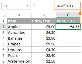
Tip. By default, all cell references in Excel are relative references. So, when writing a formula, you can add a relative reference by clicking the corresponding cell on the worksheet instead of typing a cell reference manually.
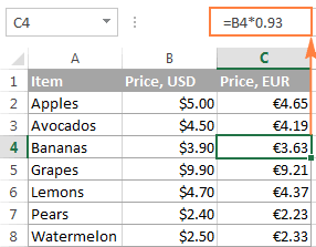
To copy the formula down the column, hover the mouse over the fill handle (a small square in the bottom-right corner of the selected cell). As you do this, the cursor will change to a thin black cross, and you hold and drag it over the cells you want to auto-fill.

That's it! The formula is copied to other cells with relative references that are adjusted properly for each individual cell. To make sure that a value in each cell is calculated correctly, select any of the cells and view the formula in the formula bar. In this example, I've selected cell C4, and see that the cell reference in the formula is relative to row 4, exactly as it should be:
Excel absolute cell reference (with $ sign)
An absolute reference in Excel is a cell address with the dollar sign ($) in the row or column coordinates, like $A$1.
The dollar sign fixes the reference to a given cell, so that it remains unchanged no matter where the formula moves. In other words, using $ in cell references allows you to copy the formula in Excel without changing references.

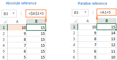
For example, if you have 10 in cell A1 and you use an absolute cell reference ($A$1), the formula =$A$1+5 will always return 15, no matter what other cells that formula is copied to. On the other hand, if you write the same formula with a relative cell reference (A1), and then copy it down to other cells in the column, a different value will be calculated for each row. The following image demonstrates the difference:
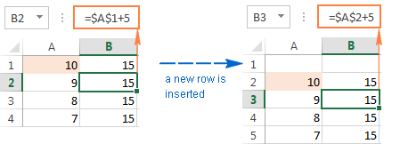
Note. Though we have been saying that an absolute reference in Excel never changes, in fact it does change when you add or remove rows and/or columns in your worksheet, and this changes the location of the referenced cell. In the above example, if we insert a new row at the top of the worksheet, Excel is smart enough to adjust the formula to reflect that change:
In real worksheets, it's a very rare case when you'd use only absolute references in your Excel formula. However, there are a lot of tasks that require using both absolute and relative references, as demonstrated in the following examples.
Note. An absolute cell reference should not be confused with absolute value, which is the magnitude of a number without regard to its sign.
Using relative and absolute cell references in one formula
Quite often you may need a formula where some cell references are adjusted for the columns and rows where the formula is copied, while others remain fixed on specific cells. In other words, you have to use relative and absolute cell references in a single formula.
Example 1. Relative and absolute cell references for calculating numbers
In our previous example with USD and EUR prices, you may not want to hardcode the exchange rate in the formula. Instead, you can enter that number in some cell, say C1, and fix that cell reference in the formula by using the dollar sign ($) like shown in the following screenshot:
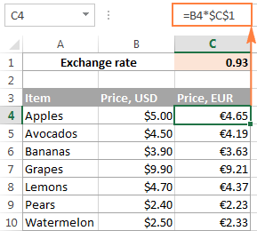
In this formula (B4*$C$1), there are two cell reference types:
- B4 - relative cell reference that is adjusted for each row, and
- $C$1 - absolute cell reference that never changes no matter where the formula is copied.
An advantage of this approach is that your users can calculate EUR prices based on a variable exchange rate without changing the formula. Once the conversion rate changes, all you have to do is to update the value in cell C1.
Example 2. Relative and absolute cell references for calculating dates
Another common use of absolute and relative cell references in a single formula is Calculating dates in Excel based on today's date.
Supposing you have a list of delivery dates in column B, and you input the current date in C1 by using the TODAY() function. What you want to know is in how many days each item ships, and you can calculate this out by using the following formula: =B4-$C$1
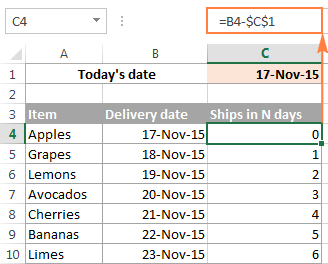
And again, we use two reference types in the formula:
- Relative for the cell with the first delivery date (B4), because you want this cell reference to vary depending on the row where the formula resides.
- Absolute for the cell with today's date ($C$1), because you want this cell reference to remain constant.
Wrapping up, whenever you want to create an Excel static cell reference that always refers to the same cell, be sure to include the dollar sign ($) in your formula to create an absolute reference in Excel.
Excel mixed cell reference
A mixed cell reference in Excel is a reference where either the column letter or a row number is fixed. For example, $A1 and A$1 are mixed references. But what does each mean? It's very simple.
As you remember, an Excel absolute reference contains 2 dollar signs ($) that lock both the column and the row. In a mixed cell reference, only one coordinate is fixed (absolute) and the other (relative) will change based on a relative position of the row or column:
- Absolute column and relative row, like $A1. When a formula with this reference type is copied to other cells, the $ sign in front of the column letter locks the reference to the specified column so that it never changes. The relative row reference, without the dollar sign, varies depending on the row to which the formula is copied.
- Relative column and absolute row, like A$1. In this reference type, it's the row's reference that won't change, and the column's reference will.

Below you will find an example of using both mixed cell reference types that will hopefully make things easier to understand.
Using a mixed reference in Excel - formula example
For this example, we will be using our currency conversion table again. But this time, we won't limit ourselves only to the USD - EUR conversion. What we are going to do is to convert the dollar prices to a number of other currencies, all with a single formula!
To begin with, let's enter the conversion rates in some row, say row 2, as shown in the screenshot below. And then, you write just one formula for the top-left cell (C5 in this example) to calculate the EUR price:
=$B5*C$2
Where $B5 is the dollar price in the same row, and C$2 is the USD - EUR conversion rate.
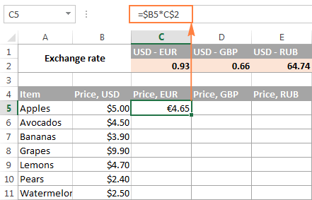
And now, copy the formula down to other cells in column C, and after that auto-fill other columns with the same formula by dragging the fill handle. As the result, you will have 3 different price columns calculated correctly based on the corresponding exchange rate in row 2 in the same column. To verify this, select any cell in the table and view the formula in the formula bar.
For example, let's select cell D7 (in the GBP column). What we see here is the formula =$B7*D$2 that takes a USD price in B7 and multiplies it by the value in D2, which is the USD-GBP conversion rate, just what the doctor ordered :)

And now, let's understand how it comes that Excel exactly knows which price to take and which exchange rate to multiply it by. As you may have guessed, it's the mixed cell references that do the trick ($B5*C$2).
- $B5 - absolute column and relative row. Here you add the dollar sign ($) only before the column letter to anchor the reference to column A, so Excel always uses the original USD prices for all conversions. The row reference (without the $ sign) is not locked because you want to calculate the prices for each row individually.
- C$2 - relative column and absolute row. Because all the exchange rates reside in row 2, you lock the row reference by putting the dollar sign ($) in front of the row number. And now, no matter what row you copy the formula to, Excel will always look for the exchange rate in row 2. And because the column reference is relative (without $ sign), it will get adjusted for the column to which the formula is copied.
How to reference an entire column or row in Excel
When you are working with an Excel worksheet that has a variable number of rows, you may want to refer to all of the cells within a specific column. To reference the whole column, just type a column letter twice and a colon in between, for example A:A.
A whole-column reference
As well as cell references, an entire column reference can be absolute and relative, for example:
- Absolute column reference, like $A:$A
- Relative column reference, like A:A
And again, you use the dollar sign ($) in an absolute column reference to lock it to a certain column, for the entire-column reference not to change when you copy a formula to other cells.
A relative column reference will change when the formula is copied or moved to other columns and will remain intact when you copy the formula to other cells within the same column.
A whole-row reference
To refer to the entire row, you use the same approach except that you type row numbers instead of column letters:
- Absolute row reference, like $1:$1
- Relative row reference, like 1:1
In theory, you can also create a mixed entire-column reference or mixed entire-row reference, like $A:A or $1:1, respectively. I say "in theory", because I cannot think of any practical application of such references, though Example 4 proves that formulas with such references work exactly as they are supposed to.
Example 1. Excel entire-column reference (absolute and relative)
Supposing you have some numbers in column B and you want to find out their total and average. The problem is that new rows are added to the table every week, so writing a usual SUM() or AVERAGE() formula for a fixed range of cells is not the way to go. Instead, you can reference the entire column B:
=SUM($B:$B) - use the dollar sign ($) to make an absolute whole-column reference that locks the formula to column B.
=SUM(B:B) - write the formula with no $ to make a relative whole-column reference that will get changed as you copy the formula to other columns.
Tip. When writing the formula, click the column letter to have the entire-column reference added to the formula. As is the case with cell references, Excel inserts a relative reference (with no $ sign) by default:

In the same fashion, we write a formula to calculate the average price in the whole column B:
=AVERAGE(B:B)
In this example, we are using a relative entire-column reference, so our formula gets adjusted properly when we copy it to other columns:

Note. When using an entire-column reference in your Excel formulas, never input the formula anywhere within the same column. For example, it might seem like a good idea to enter the formula =SUM(B:B) in one of the empty bottom-most cells in column B to have the total at the end of the same column. Don't do this! This would create a so-called circular reference and the formula would return 0.
Example 2. Excel entire-row reference (absolute and relative)
If the data in your Excel sheet is organized in rows rather than columns, then you can reference an entire row in your formula. For example, this is how we can calculate an average price in row 2:
=AVERAGE($2:$2) - an absolute whole-row reference is locked to a specific row by using the dollar sign ($).
=AVERAGE(2:2) - a relative whole-row reference will change when the formula is copied to other rows.
In this example, we need a relative entire-row reference because we have 3 rows of data and we want to calculate an average in each row by copying the same formula:

Example 3. How to refer to an entire column excluding the first few rows
This is a very topical problem, because quite often the first few row in a worksheet contain some introductory clause or explanatory information and you don't want to include them in your calculations. Regrettably, Excel does not allow references like B5:B that would include all the rows in column B beginning with row 5. If you try adding such a reference, your formula will most likely return the #NAME error.
Instead, you can specify a maximum row, so that your reference includes all possible rows in a given column. In Excel 2016, 2013, 2010, and 2007, a maximum is 1,048,576 rows and 16,384 columns. Earlier Excel versions have a row maximum of 65,536 and column maximum of 256.
So, to find an average for each price column in the below table (columns B through D), you enter the following formula in cell F2, and then copy it to cells G2 and H2:
=AVERAGE(B5:B1048576)
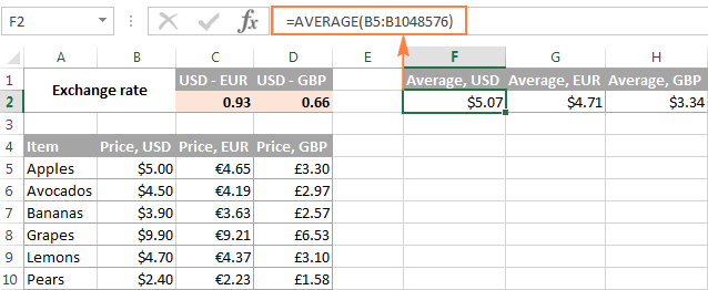
If you are using the SUM function, you can also subtract the rows you want to exclude:
=SUM(B:B)-SUM(B1:B4)
Example 4. Using a mixed entire-column reference in Excel
As I mentioned a few paragraphs before, you can also make a mixed entire-column or entire-row reference in Excel:
- Mixed column reference, like $A:A
- Mixed row reference, like $1:1
Now, let's see what happens when you copy a formula with such references to other cells. Supposing you input the formula =SUM($B:B) in some cell, F2 in this example. When you copy the formula to the adjacent right-hand cell (G2), it changes to =SUM($B:C) because the first B is fixed with the $ sign, while the second isn't. As the result, the formula will add up all the numbers in columns B and C. Not sure if this has any practical value, but you may want to know how it works:

A word of caution! Don't use too many entire column/row references in a worksheet because they may slow down your Excel.
How to switch between absolute, relative, and mixed references (F4 key)
When you write an Excel formula, $ sign can of course be typed manually to change a relative cell reference to absolute or mixed. Or, you can hit the F4 key to speed things up. For the F4 shortcut to work, you have to be in formula edit mode:
- Select the cell with the formula.
- Enter Edit mode by pressing the F2 key, or double-click the cell.
- Select the cell reference you want to change.
- Press F4 to toggle between four cell reference types.
If you've selected a relative cell reference with no $ sign, like A1, repeatedly hitting the F4 key toggles between an absolute reference with both dollar signs like $A$1, absolute row A$1, absolute column $A1, and then back to the relative reference A1.

Note. If you press F4 without selecting any cell reference, the reference to the left of the mouse pointer will get selected automatically and changed to another reference type.
I hope now you fully understand what relative and absolute cell references are, and an Excel formula with $ signs is no longer a mystery. In the next few articles, we will continue learning various aspects of Excel cell references such as referencing another worksheet, 3d reference, structured reference, circular reference, and so on. In the meantime, I thank you for reading and hope to see you on our blog next week!
 by
by
98 comments
Thank you!!!!
I finally found the way to copy formulas, so that part of the formula won't move with $A$1 command. This is a huge time saver for me!
Hi,
Nice walkthrough,
I however has another issue:
I write a reference in a stationary cell, lets say =SUM(A5:A25).
The area A5:A25 is marked to take user input, but because of different reasons the users will probably use "inser new row" at A5, pushing everything below down one step. This makes the reference move too, putting the new row outside of the function. I tried finding a way of defining the reference as a string rather than a direct reference but has not found a way that Excel will allow. The only way that works so far is to reference the whole column (A:A), but that of course but some limits on where you can put other necessary data.
Any thoughts?
And thanks in advance for any help you can give.
Hi! You can lock a reference to a range of cells using the INDIRECT function. Read more: Using Excel INDIRECT function to lock a cell reference. For example:
=SUM(INDIRECT("A5:A25"))
You can also convert your data into an Excel table and make the SUM formula refer to a column in that spreadsheet, as described here: Structured references in Excel tables.
Extremely helpful and clear. To the point. Keep it up!
Hi,
this was incredibly helpful but I have one question/problem. I have a large excel spreadsheet to track speakers at a conference. I have mutiple tabs that are statistics for region, gender, topics etc.
So basically, let's say I lock a cell in my forumla as E$2 this means that when I copy the formula down the cells, the reference will not change as the row number is locked. But I want the column to change as it moves down but this isn't happening. Can you explain/find a solution? If I copy the formula to the right, the column alphabet would change as it’s not locked but this is not helpful so I don't understand why Excel applies two different rules to the same cell forumulation (i.e. E$2).
Thanks.
Hi!
When moving down, you stay in the same column. Why should he change?
Hi,
I may missed this is your write up but i can't get excel to add coloumns with XLOOKUP, my formula is
=XLOOKUP(Sheet1!$B$3,Sheet2!$A$2:$A$3,Sheet2!B$2:B$3,"")
as you can see i've locked all rows and coloumns except in the return array as i want the coloumns in that to go up letter by letter but excel wont do it
Can you help?
Hi!
If you want to copy the formula down the column and look for new values, use a relative reference in the first argument.
Hi Sorry i forgot to add this is when i drag the autofill...i want the columns in the return array to automatically go up
Thank you
Hi,
I understand whats happening...my Sheet1 has a list of products vertically and Sheet2 has them horzontally...what i'm trying to do is drag the autofill downwords and have it increase the columns...doesnt work but if i drag if horizontally it does work
So my question now is...is it possible to do what i want or do i have to redo my sheet?
Wow.. Amazing.
What a knowledge you have... Everything is explained very simple, clearly & in detail.
Thank you for great opportunity to learn these formulas it is very helpful to us who seek ideas or knowledge about these things,thank you for the team who made effort to creat and published here on webpage
how to use IFS , in statement, i have the system reset which is equal to 1, hardware reset is equal to 2, then software system is equal to 3
Hi!
You can learn more about IFS function in Excel in this article on our blog.
The fact I am still at the very beginning of Excel course and I am just embraced. I feel it is gonna be friendly and let my mind work a lot.
Thanks for your great work!
God bless you for this
How do you set up a formula to reference a cell in the same column when a new column is added to the 'left'? e.g. Cell D4 contains =IF(J4="";"";J4) where column J contains purchases made today. When purchases are made on a new day, the new day's purchases are in Column J and the previous day's purchases are shifted to Column K. How do I set up Cell D4 to reference J4
Hello!
Use absolute cell references in your formulas.
Excellent. Thanks for the very informative blog.
In a question for school they ask us to give an aswer to something like formula 5^(1+4)*4-5/7 using the order calculation followed by excel. Round to two decimal, and use a decimal (“.”). What is the function of ("."). Thanks in advance for your help.
Hi!
I recommend reading this guide: Rounding in Excel: ROUND, ROUNDUP, ROUNDDOWN, FLOOR ...
Please refer to attached excel sheet in which Bill of material is created. The cell L3 is multiplication factor of j3 and k3. Since k1 to k13 is merged we have used dollar symbol so that k3 link will not change.
But when this set is copied for next beam set ie 1 to 13 of beam 1 to beam 2 the link is again k3 only. Is there any solution for that.
If we remove dollar symbol k3 is increasing in steps of k4,k5,k6 which is not acceptable.
what does the ^ mean in excel?
Hello!
Please have a look at this article — Operators used in Excel spreadsheet formulas
I hope my advice will help you solve your task.
Best Explanation...
This was a life-saver, I always get so confused about this but this article manages to break it down in a way that makes me understand the concept easily! thank you
Hello, I have been wondering before how to go about the use of dollar sign in excel formulas. This has been the best explanation I have ever gotten in excel study. From nothing and in a few minutes I've already understood!!!. I will say thanks so much for preparing this article.
How can i fellow your regular post
This is very insightful
complicated