This short tutorial explains the basics of Excel circular reference and why you should beware of using them. You will also learn how to check, find and remove circular references in Excel worksheets, and if none of the above is an option, how to enable and use circular formulas.
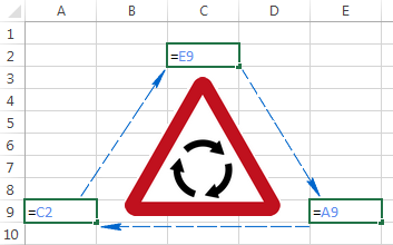
You've tried to enter some formula in your Excel sheet, but for some reason it's not working. Instead, it tells you something about a circular reference. Is this how you ended up on this page? :)
Thousands of users are facing the same problem on a daily basis simply because of forcing an Excel formula to calculate its own cell. When you try to do this, Excel throws up the following error message:
"Careful, we found one or more circular references in your workbook which might cause your formula to calculate incorrectly."
To put it simply, what Excel is trying to say is this: "Hey, I may get stuck at the round-about. Are you sure you want me to proceed anyway?"
As you can understand, circular references in Excel are troublesome, and the common sense says to avoid them whenever possible. However, there may be some rare cases when an Excel circular reference is the only possible solution for the task you are faced with.
What is a circular reference in Excel?
Here is a very straight and concise definition of a circular reference provided by Microsoft:
"When an Excel formula refers back to its own cell, either directly or indirectly, it creates a circular reference."
For instance, if you select cell A1 and type =A1 in it, this would create an Excel circular reference. Entering any other formula or calculation referring to A1 would have the same affect, e.g. =A1*5 or =IF(A1=1, "OK").
As soon as you hit Enter to complete such a formula, you'll get the following warning message:
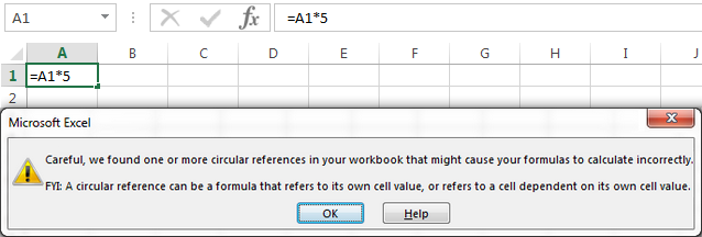
Why does Microsoft Excel give you a heads-up? Because Excel circular references can iterate indefinitely creating an endless loop, thus significantly slowing down the workbook calculations.
Once you got the above warning, you can click Help for more information, or close the message window by clicking either OK or the cross button. When you close the message window, Excel displays either a zero (0) or the last calculated value in the cell. Yep, in some cases, a formula with a circular reference can complete successfully before it tries to calculate itself, and when that happens, Microsoft Excel returns the value from the last successful calculation.
Note. In many cases, when you enter more than one formula with a circular reference, Excel doesn't display the warning message repeatedly.
But why would anyone want to make such a stupid formula that does nothing but cause unnecessary problems? Right, no sane user would ever want to intentionally input a circular formula like the above one. However, you may create a circular reference in your Excel sheet accidentally, and here's a very common scenario.
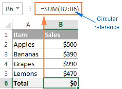
Supposing you want to add up values in column A with a usual SUM formula, and when doing this you inadvertently include the total cell itself (B6 in this example).
If circular references are not allowed in your Excel (and they are turned off by default), you will see an error message we've discussed a moment ago. If iterative calculations are turned on, then your circular formula will return 0 like in the following screenshot:
In some cases, one or more blue arrows can also appear in your spreadsheet all of a sudden, so you might think your Excel has gone mad and is about to crash.
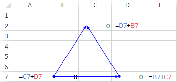
In fact, those arrows are nothing more than Trace Precedents or Trace Dependents, which indicate which cells affect or are affected by the active cell. We will discuss how you can show and hide these arrows a bit later.
By now, you might have an impression that Excel circular references are a worthless and dangerous thing, and may wonder why Excel has not banned them altogether. As already mentioned, there are some very rare cases when using a circular reference in Excel can be justified because it provides a shorter and more elegant solution, if not the only possible one. The following example demonstrates such a formula.
Using an Excel circular reference - formula example
In one of our previous tutorials, we discussed how to insert today's date in Excel. And an overwhelming majority of questions posted in comments were about how to enter a timestamp in Excel without it changing every time the worksheet is reopened or recalculated. I was very hesitant to reply to those comments because the only solution I know involves circular references, and they should be treated with care. Anyway, here is a very common scenario...
Supposing you have a list of items in column A, and you enter the delivery status in column B. As soon as you type "Yes" in column B, you want the current date and time to be automatically inserted in the same row in column C as a static unchangeable timestamp.
Using a trivial NOW() formula is not an option because this Excel function is volatile, meaning that it updates its value every time the worksheets is re-opened or recalculated. A possible solution is using nested IF functions with a circular reference in the second IF:
=IF(B2="yes", IF(C2="" ,NOW(), C2), "")
Where B2 is the delivery status, and C2 is the cell where you want a timestamp to appear.
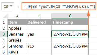
In the above formula, the first IF function checks cell B2 for "Yes" (or any other text you supply to the formula), and if the specified text is there, it runs the second IF, otherwise returns an empty string. And the second IF function is a circular formula that fetches the current day and time if C2 doesn't already have a value in it, thus saving all existing time stamps.
Note. For this Excel circular formula to work, you should allow iterative calculations in your worksheet, and this is exactly what we are going to discuss next.
How to enable / disable circular references in Excel
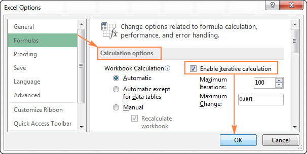
As noted earlier, iterative calculations are usually turned off in Excel be default (in this context, iteration is the repeated recalculation until a specific numeric condition is met). For circular formulas to work, you must enable iterative calculations in your Excel workbook.
In Excel 2010 and higher, click File > Options, go to Formulas, and select the Enable iterative calculation check box under the Calculation options section.
In Excel 2007, click Office button > Excel options > Formulas > Iteration area.
In Excel 2003 and earlier, the Iterative Calculation option resides under Menu > Tools > Options > Calculation tab.
When you turn on iterative calculations, you must specify the following two options:
- Maximum Iterations box - specifies how many times the formula should recalculate. The higher the number of iterations, the more time the calculation takes.
- Maximum Change box - specifies the maximum change between calculation results. The smaller the number, the more accurate result you get and the more time Excel takes to calculate the worksheet.
The default settings are 100 for Maximum Iterations, and 0.001 for Maximum Change. What it means is that Microsoft Excel will stop calculating your circular formula after 100 iterations or after a less than 0.001 change between iterations, whichever comes first.
Why you should avoid using circular references in Excel
As you already know, using circular references in Excel is a slippery and not recommended approach. Apart from performance issues and a warning message displayed on every opening of a workbook (unless iterative calculations are on), circular references can lead to a number of other issues, which are not immediately apparent.
For example, if you select a cell with a circular reference, and then accidentally switch to the formula editing mode (either by pressing F2 or double-clicking the cell), and then you press Enter without making any changes to the formula, it will return zero.
So, here's a word of advice from many respected Excel gurus - try to avoid circular references in your sheets whenever possible.
How to find circular references in Excel
To check your Excel workbook for circular references, perform the following steps:
- Go to the Formulas tab, click the arrow next to Error Checking, and point to Circular References The last entered circular reference is displayed there.
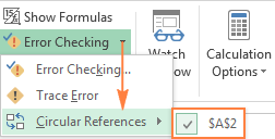
- Click on the cell listed under Circular References, and Excel will bring you exactly to that cell.
As soon as you do this, the status bar will notify you that circular references are found in your workbook and display an address of one of those cells:
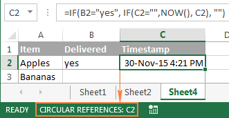
If circular references are found in other sheets, the status bar displays only "Circular References" with no cell address.
Note. This feature is disabled when the Iterative Calculation option is turned on, so you need to turn it off before you start checking the workbook for circular references.
How to remove circular references in Excel
Regrettably, there is no mechanism in Excel that would let you eliminate all circular formulas in a workbook on a button click. To get rid of them, you will have to inspect each circular reference individually by performing the above steps, and then either remove a given circular formula altogether or replace it with one or more simple formulas.
How to trace relationships between formulas and cells
In cases when an Excel circular reference is not obvious, the Trace Precedents and Trace Dependents features can give you a clue by drawing one or more lines that show which cells affect or are affected by the selected cell.
To display the trace arrows, go to the Formulas tab > Formula Auditing group, and click one of the options:
Trace Precedents - traces cells that provide data to a formula, i.e. draws lines indicating which cells affect the selected cell.
Trace Dependents - traces cells that are dependent on the active cell, i.e. draws lines indicating which cells are affected by the selected cell. In other words, it shows which cells contain formulas that reference the selected cell.
Alternatively, you can use the following shortcuts:
- Trace Precedents: Alt+T U T
- Trace Dependents: Alt+T U D
To hide the arrows, click the Remove Arrows button that resides right underneath Trace Dependents.
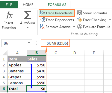
In the above example, the Trace Precedents arrow shows which cells directly supply data to B6. As you can see, cell B6 is also included, which makes it a circular reference and cause the formula to return zero. Of course, this one is easy to fix, just replace B6 with B5 in SUM's argument: =SUM(B2:B5)
Other circular references might not be that obvious and require more thought and calculations.
This is how you deal with Excel circular references. Hopefully, this short tutorial has shed some light on this "blind spot", and now you can do further research to learn more. I thank you for reading and look forward to seeing you on our blog next week!
 by
by
34 comments
Thank you very much now i can find the error in my workbook easily.
Hey! Thanks for this education. I got the whole stuff. But how did you format the date?
Hi! I recommend reading this guide: How to change Excel date format and create custom formatting.
I am trying to populate cells with cut lengths on parts. I got it where it sorts the lengths from greatest to shortest, it will also calculate the number of pcs that are a certain length. there is a lot to it to say the least. the following is the formula i am trying to use but it is giving me a circular reference error:
IFS(AND(I7=G7)=TRUE,G7,AND(I8G8)=TRUE,G8,AND(I9G9)=TRUE,G9,AND(I10G10)=TRUE,G10,AND(I11G11)=TRUE,G11,AND(I12G12)=TRUE,H12,AND(I13G13)=TRUE,H13,AND(I14G14)=TRUE,H14,AND(I15G15)=TRUE,H15,AND(I16G16)=TRUE,G16).
=IFS(AND(I7=G7)=TRUE,G7,AND(I8G8)=TRUE,G8,AND(I9G9)=TRUE,G9,AND(I10G10)=TRUE,G10,AND(I11G11)=TRUE,G11,AND(I12G12)=TRUE,H12,AND(I13G13)=TRUE,H13,AND(I14G14)=TRUE,H14,AND(I15G15)=TRUE,H15,AND(I16G16)=TRUE,G16)
It did not paste right for some reason on the original
formula will not paste write in comments,
Okay, but then what alternative would you then suggest to simplify: =IF(A10<>"",IF(B10="",NOW(),B10),""). I use this formula to automatically enter the date of the data entry. It's extremely important to have this information pull through correctly. Also, is there a work around for 365 (excel online) as this function does not work at all or is not supported in Excel online (Or so it seems)
Hi! To prevent your date from changing automatically, in addition to the method you described, you can use several methods:
1. Use Shortcuts to insert the current date and time
2. Replace the date and time returned by the TODAY function with their values. Copy the date (CTRL + C), then paste only the values using Paste Special or Shortcut CTRL + ALT + V.
3. Use VBA macro, to automatically insert current date when cell value changes.
I am writing a employee roster.
What formula can I use to replace a circular formula which states e.g., if tally of shifts <= to X, then plot shift.
The cell which 'counts (tallies)' the number of shifts already plotted does not increase by 1, when the above formula is true.
Is there an alternative formula I could use?
Unfortunately, this information is not enough to recommend a formula to you.
Hi I am trying to use the timestamp function but in a different way. I have a field for my PO number and then a Vlookup to pull through the due date however once the purchase order is closed off it will no longer be available in my table. what i was trying to do is if the Vlookup failed to find the due date then it left the old data in there. for example PO 125846 due 24/1/22
I used formula =IF(E4>0,IF(A4"",A4,Vlookup(E4,'Shortages SQL'!$A:$R,16,FALSE))
where E4 = the PO Number
A4 = feild for the due date
vlookup from 'Shortages SQL" tab to pull through due date if one is not already there
When the PO due date already exists it changes to 0/01/1900 instead of keeping the date that was there e.g 24/1/22
how can i make it keep the 24/1/22 ?
thanks
Sorry just thought that i would add i have set excel to Enable iterative calculations
Say A1 has new purchases and B1 has qty in stock.. how can B1 automatically update anytime I enter a new figure in A1.
Hi!
If B1 contains a formula, then add minus A1 to it. If a number is written in B1, then it cannot be changed using a formula.
I am trying to set four cells so that they can only contain "Yes" or "No" but only one can be "Yes" at any one time, changing one of the "No" values to "Yes" needs to make the other cell switch to "No", then I need to protect this so that nothing else can be entered into the cells. Easy to make this work with two cells but is there a way with four?
Please can you help.
Regards
Hello!
You can use Data Validation rule
=COUNTIF(B1:B4,"Yes")<2
Set it for each of the four cells.
The automatic change of the cell value from Yes to No is possible only with a VBA macro.
If you want the current time stamp there's a simple shortcut Ctrl + ; or for a time stamp you can do Ctrl + Shift + ;
Current Date = Ctrl + ;
Current Time = Shift + Ctrl + ;
Whoops
Hello -
I have a question about the above formula =IF(B2="yes", IF(C2="" ,NOW(), C2), "").
The sample shows that the dates are the same but the times are different. I follow the above formula but when I go to enter yes, the whole column changes to the same time. And to better help, here's what I'm trying to do:
I'm going to work in a stockroom and want to make it more productive and have an easier managing system for items than what's currently being used. I want to create a spread sheet where I can keep track of the date/time products enter or leave. For example, say Johnny is taking out a ream of paper on 4-3-19 at 3:50pm. Susie comes the same date but at 4:00pm and takes out 2 staplers. How can I get it to show the 3:50pm time and the 4:00pm with the current date?
Can you check time zone and Pc Current Date & Time
I've used =NOW()to insert the current date into a cell
for years. In the latest version of Office 365 Excel it generates a circular reference error at every occurrence and shuts down the application even though it appears to be accepting inputs to new cells. Is anyone else experiencing this issue?
did you ever get an answer?
Thank you soooooooooo much , it solved my problem completely.
I am getting a message while putting formulas in Microsoft excel 7 sheets that there "exists circular reference" in the sheet and the formula that I am trying to put is not calculating anything and showing me the same message every time so how to solve this problem if you can help me to solve the problem i will really appreciate your replies
I keep getting false circular reference errors. What could cause that?
Hi Greg,
Usually, Excel displays that error when there is one or more formula on a sheet that directly or indirectly references its own cell. A typical example is a formula, say, in A10: =SUM(A:A)
This problem can be solved if you use IFERROR function
how?
Hi, when I use this =IF(B2="yes", IF(C2="" ,NOW(), C2), "") , I get 1/0/1900 as the timestamp. I have enabled iterative calculation. why am I not getting the right time stamp?
same here.. do you find the right formula? may i know it?
Try to put "" instead of "=" on the first IF statement. See sample below.
=IF(C5"",(IF(D5="",NOW(),D5)),"")
" "
For about 20 years I have been calculating our budget with a simple system. I have rows named 'housekeeping', 'vehicle expenses', 'insurance', 'medical expenses', 'clothing', ‘holiday & family’, ‘savings’ and a host of other items we budget for.
The formula was simple, column 1 would have the name of budget, column 2 and 3 would be blank, that’s where we enter amount budgeted and spent for each item, like debit and credit columns. There is a hidden column (4) where we calculate the sum of column 3 less 2 (income less expenditure). Column 5 would calculate the balance of column 4 (which could be a plus or minus amount), plus column 5, (a circular reference) which would give us a running balance of that row. We delete entries in columns 2 and 3 and the balance remains for the following session. All the items added together in column 5 would then correspond with our bank statement.
Through the years this system worked flawless until Microsoft brought out Excel 2016. The programme now refuses to calculate the circular reference and I don’t know how to get around this.
Has anyone got any suggestions to get around the circular reference?
You can use a simple macro, which allows a statements such as this:
x = x + y