In this tutorial, you will learn how to automatically highlight duplicates in Excel once something has been typed. We are going to have a close look at how to shade duplicate cells, entire rows, or consecutive dupes using conditional formatting and a special tool.
Last week, we explored different ways to identify duplicates in Excel with formulas. Undoubtedly, those solutions are very useful, but highlighting duplicate entries in a certain color could make data analysis even easier.
The fastest way to find and highlight duplicates in Excel is using conditional formatting. The biggest advantage of this method is that it not only shows dupes in the existing data but automatically checks new data for duplicates right when you enter it in a worksheet.
These techniques work in all versions of Excel 365, Excel 2021, Excel 2019, Excel 2016, Excel 2013, Excel 2010 and lower.
How to highlight duplicates in Excel
In all Excel versions, there is a predefined rule for highlighting duplicate cells. To apply this rule in your worksheets, perform the following steps:
- Select the data you want to check for duplicates. This can be a column, a row or a range of cells.
- On the Home tab, in the Styles group, click Conditional Formatting > Highlight Cells Rules > Duplicate Values…

- The Duplicate Values dialog window will open with the Light Red Fill and Dark Red Text format selected by default. To apply the default format, simply click OK.
Apart from the red fill and text formatting, a handful of other predefined formats are available in the dropdown list. To shade duplicates using some other color, click Custom Format… (the last item in the drop-down) and select the fill and/or font color of your liking.

Tip. To highlight unique values, select Unique in the left-hand box.
Using the inbuilt rule, you can highlight duplicates in one column or in several columns as shown in the following screenshot:

Note. When applying the built-in duplicate rule to two or more columns, Excel does not compare the values in those columns, it simply highlights all duplicate instances in the range. If you want to find and highlight matches and differences between 2 columns, follow the examples in the above linked tutorial.
When using Excel's inbuilt rule for highlighting duplicate values, please keep in mind the following two things:
- It works only for individual cells. To highlight duplicate rows, you would need to create your own rules either based on values in a specific column or by comparing values in several columns.
- It shades duplicate cells including their first occurrences. To highlight all duplicates except first instances, create a conditional formatting rule based on formula as explained in the next example.
How to highlight duplicates without 1st occurrences
To highlight 2nd and all subsequent duplicate occurrences, select the cells you want to color, and create a formula-based rule in this way:
- On the Home tab, in the Styles group, click Conditional Formatting > New rule > Use a formula to determine which cells to format.
- In the Format values where this formula is true box, enter a formula similar to this:
=COUNTIF($A$2:$A2,$A2)>1Where A2 is the top-most cell of the selected range.
- Click the Format… button and select the fill and/or font color you want.
- Finally, click OK to save and apply the rule.
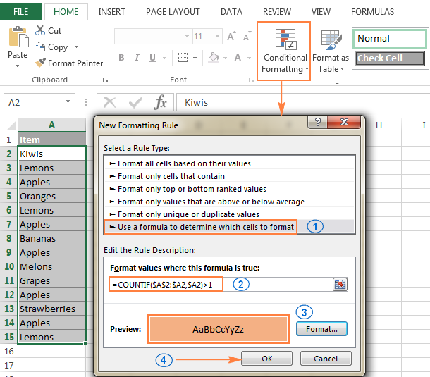
If you don't have much experience with Excel conditional formatting, you will find the detailed steps to create a formula-based rule in the following tutorial: Excel conditional formatting based on another cell value.
As the result, the duplicate cells excluding first instances will get highlighted with the color of your choosing:

How to show 3rd, 4th and all subsequent duplicate records
To view duplicates beginning with the Nth occurrence, create a conditional formatting rule based on the formula like in the previous example, with the only difference that you replace >1 at the end of the formula with the required number. For example:
To highlight 3rd and all subsequent duplicate instances, create a conditional formatting rule based on this formula:
=COUNTIF($A$2:$A2,$A2)>=3
To shade4th and all subsequent duplicate records, use this formula:
=COUNTIF($A$2:$A2,$A2)>=4
To highlight only specific occurrences, use the equal to operator (=). For example, to highlight only 2nd instances, you would go with this formula:
=COUNTIF($A$2:$A2,$A2)=2
How to highlight duplicates in a range (multiple columns)
When you want to check for duplicates over multiple columns, not by comparing the columns to each other, but find all instances of the same item in all the columns, use one of the following solutions.
Highlight duplicates in multiple columns including 1st occurrences
If the first instance of an item that appears in the data set more than once is deemed a duplicate, the easiest way to go is use Excel's built-in rule for duplicates.
Or, create a conditional formatting rule with this formula:
For example, to highlight duplicates in the range A2:C8, the formula goes as follows:
=COUNTIF($A$2:$C$8, A2)>1
Please notice the use of absolute cell references for the range ($A$2:$C$8), and relative references for the top cell (A2).

Highlight duplicates in multiple columns except 1st occurrences
The solution for this scenario is a lot trickier, no wonder Excel has no built-in rule for it :)
To highlight duplicate entries in several columns ignoring the 1st occurrences, you will have to create 2 rules with the following formulas:
Rule 1. Applies to the first column
Here you use exactly the same formula as we used to highlight duplicates without 1st occurrences in one column (the detailed steps can be found here).
In this example, we are creating a rule for A2:A8 with this formula:
=COUNTIF($A$2:$A2,$A2)>1
As the result, the duplicate items without 1st occurrences are highlighted in the left-most column of the range (there is only one such item in our case):

Rule 2. Applies to all subsequent columns
To highlight duplicates in the remaining columns (B2:C8), use this formula:
=COUNTIF(A$2:$A$8,B2)+COUNTIF(B$2:B2,B2)>1
In the above formula, the first COUNTIF function counts the occurrences of a given item in the first column, and the second COUNTIF does the same for all subsequent columns. And then, you add up those numbers and check if the sum is greater than 1.
As the result, all duplicated items excluding their 1st occurrences are found and highlighted:

Highlight duplicates in all columns with a single rule
Another possible solution is to add an empty column to the left of your dataset, and combine the above formulas into a single formula like this:
=IF(COLUMNS($B2:B2)>1,COUNTIF(A$2:$B$8,B2),0) + COUNTIF(B$2:B2,B2)>1
Where B2 is the top cell with data in the 2nd column of the target range.

To better understand the formula, let's break it down into 2 main parts:
- For the first column (B), the IF condition is never met, so only the second COUNTIF function is calculated (we have used this formula to find duplicates except first occurrences in one column).
- For all subsequent columns (C2:D8), the key point is the clever use of absolute and relative references in the two COUNTIF functions. To make things easier to understand, I've copied it to column G, so you can see how the formula changes when applied to other cells:

Because the IF condition is always TRUE for all the columns other than the first one (number of columns is greater than 1), the formula proceeds in this way:
- Counts the number of occurrences of a given item (D5 in the screenshot above) in all columns to the left of the given column:
COUNTIF(B$2:$C$8,D5) - Counts the number of a given item's occurrences in the item's column, up to the item's cell:
COUNTIF(D$2:D5,D5) - Finally, the formula adds the results of both COUNTIF functions. If the total number is greater than 1, i.e. if there is more than one occurrence of the item, the rule is applied and the item is highlighted.
Highlighting entire rows based on duplicate values in one column
If your table contains several columns, you may want to highlight whole rows based on duplicate records in a specific column.
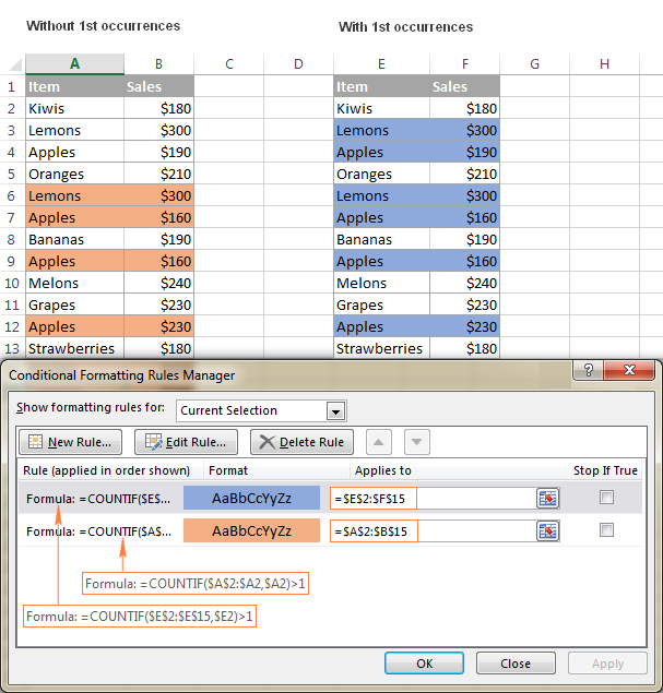
As you already know, Excel's built-in rule for duplicates works only at the cell level. But a custom formula-based rule has no problem with shading rows. The key point is to select the whole rows, and then create a rule with one of the following formulas:
- To highlight duplicate rows excluding 1st occurrences:
=COUNTIF($A$2:$A2, $A2)>1 - To highlight duplicate rows including 1st occurrences:
=COUNTIF($A$2:$A$15, $A2)>1
Where A2 is the first cell and A15 is the last used cell in the column that you want to check for duplicates. As you see, the clever use of absolute and relative cell references is what makes a difference.
The following screenshot demonstrates both rules in action:
How to highlight duplicate rows in Excel
The previous example has demonstrated how to color entire rows based on duplicate values in a specific column. But what if you want to view rows that have identical values in several columns? Or, how do you highlight absolute duplicate rows, the ones that have completely equal values in all columns?
For this, employ the COUNTIFS function that allows comparing cells by multiple criteria. For example, to highlight duplicate rows that have identical values in columns A and B, use one of the following formulas:
- To highlight duplicate rows except 1st occurrences:
=COUNTIFS($A$2:$A2, $A2, $B$2:$B2, $B2)>1 - To highlight duplicate rows with 1st occurrences:
=COUNTIFS($A$2:$A$15, $A2, $B$2:$B$15, $B2)>1
The following screenshot demonstrates the result:
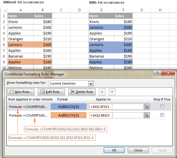
As you understand, the above example is for demonstration purposes only. When highlighting duplicate rows in your real-life sheets, you are naturally not limited to comparing values only in 2 columns, the COUNTIFS function can process up to 127 range/criteria pairs.
Highlighting consecutive duplicate cells in Excel
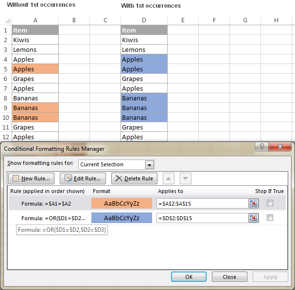
Sometimes, you may not need to highlight all duplicates in a column but rather show only consecutive duplicate cells, i.e. the ones that are next to each other. To do this, select the cells with data (not including the column header) and create a conditional formatting rule with one of the following formulas:
- To highlight consecutive duplicates without 1st occurrences:
=$A1=$A2 - To highlight consecutive duplicates with 1st occurrences:
=OR($A1=$A2, $A2=$A3)
The following screenshot demonstrates highlighting consecutive duplicate texts, but these rules will also work for consecutive duplicate numbers and dates:
If your Excel sheet may have empty rows and you don't want the consecutive blank cells to get highlighted, make the following improvements to the formulas:
- To highlight consecutive duplicate cells without 1st occurrences and ignore blank cells:
=AND($A2<>"", $A1=$A2) - To highlight consecutive duplicate cells with 1st occurrences and ignore blank cells:
=AND($A2<>"", OR($A1=$A2, $A2=$A3))
As you see, it's no big deal to highlight duplicates in Excel using conditional formatting. However, there is even a faster and easier way. To find it out, read the next section of this tutorial.
How to highlight duplicates in Excel with Duplicate Remover
The Duplicate Remover add-in is the all-in-one solution to deal with duplicate records in Excel. It can find, highlight, select, copy or move duplicated cells or entire duplicate rows.
Despite its name, the add-in can quickly highlight duplicates in different colors without deleting them.
The Duplicate Remover adds 3 new features to your Excel Ribbon:
- Dedupe Table - to immediately find and highlight duplicates in one table.
- Duplicate Remover - step-by-step wizard with advanced options to identify and highlight duplicates or unique values in 1 table.
- Compare 2 Tables - find and highlight duplicates by comparing two columns or two separate tables.
After installing Ultimate Suite for Excel, you will find these tools on the Ablebits Data tab in the Dedupe group:

Highlighting duplicates in Excel in a couple of clicks
For this example, I've created the following table with a few hundred rows. And our aim is to highlight duplicate rows that have equal values in all three columns:

Believe it or not, you can get the desired result with just 2 mouse clicks :)
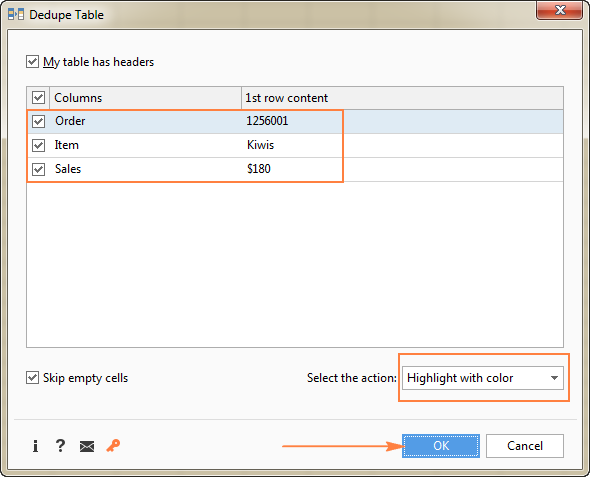
- With any cell in your table selected, click the Dedupe Table button, and the clever add-in will pick up the whole table.
- The Dedupe Table dialog window will open with all the columns selected automatically, and the Color duplicates option chosen by default. So, all you have to do is click OK :) Done!
Tip. If you want to detect duplicate rows by one or more columns, uncheck all irrelevant columns and leave only the key column(s) selected.
And the result would look similar to this:

As you see in the above image, the Dupe Table tool has highlighted duplicate rows without first instances.
If you want to highlight duplicates including first occurrences, or if you want to color unique records rather than dupes, or if you don't like the default red color, then use the Duplicate Remover wizard that has all these features and a lot of more.
Highlight duplicates in Excel using an advanced step-by-step wizard
Compared to the swift Dedupe Table tool, the Duplicate Remover wizard requires a few more clicks, but it makes up for this with a number of additional options. Let me show it to you in action:
- Select any cell within your table where you want to highlight duplicates, and click the Duplicate Remover button on the ribbon. The wizard will run and the entire table will get selected. The add-in will also suggest creating a backup copy of your table, just in case. If you don't need it, uncheck that box.
Verify that the table has been selected correctly and click Next.

- Select one of the following data types that you want to find:
- Duplicates except 1st occurrences
- Duplicates with 1st occurrences
- Unique values
- Unique values and 1st duplicate occurrences
For this example, let's find Duplicates + 1st occurrences:

- Now, select the columns to check for duplicates. Because we want to highlight complete duplicate rows, I've selected all 3 columns.

Additionally, the add-in lets you specify if your table has headers and if you want to skip empty cells. Both options are selected by default.
- Finally, choose the action to perform on duplicates. You have a number of options such as selecting, deleting, copying, moving duplicates or adding a status column to identify the dupes.
Since today we are exploring different ways to highlight duplicates in Excel, our choice is obvious :) So, select Fill with color and choose one of the standard theme colors, or click More Colors… and pick any custom RGB or HSL color.
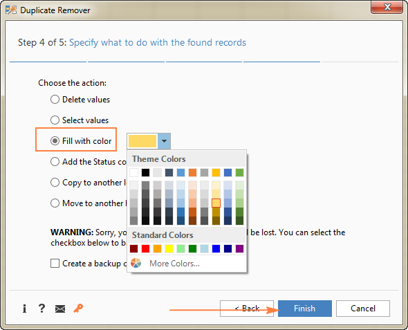
Click the Finish button and enjoy the result :)

This is how you highlight duplicates in Excel using our Duplicate Remover add-in. If you are curious to try this tool on your own worksheets, you are most welcome to download a fully-functional trial version of the Ultimate Suite that includes all our time-saving tools for Excel. And your feedback in comments will be greatly appreciated!
 by
by
86 comments
When I’m pasting data into the list it doesn’t highlight duplicates but if I type the data out it highlights. Is there a way to change this?
Hi! Please clarify your specific problem or provide additional details to highlight exactly what you need. As it's currently written, it's hard to tell exactly what you're asking.
I have a glossary in column J and I'm creating a formula to extract every occurrence of the glossary words (individual cells) that are found in column F (each cell individually, as I want a column or set of columns with all the words that match), however I have only been able to extract the first word that the formula finds, I think it needs a loop or something using LIN and MATCH, but I'm not sure -- my excel version is 2016 so I don't have some new features like FILTER and JOINTEXT -- could you assist me?
The formula thus far is:
"=IF(OR(COUNTIFS(F48,"*"&$J$1:$J$499&"*")),INDEX($J$1:$J$499,MATCH(1,COUNTIFS(F48,"*"&$J$1:$J$499&"*"),0)),"")"
Thank you very much and a Happy New Year!
Hello Cassio!
If I understand your task correctly, this article may be helpful: How to Vlookup multiple values in Excel with criteria.
Try to enter the following formula, for example, in cell E1 and then copy it down along the column:
=IFERROR(INDEX($J$1:$J$499, SMALL(IF(ISNUMBER(SEARCH($F$48,$J$1:$J$499)), ROW($J$1:$J$499),""), ROW())),"")
About " How to highlight duplicate rows in Excel" how would be the formula if the 2 columns aren't next to each other, for example if the values are in column C and Column E
Hi! Unfortunately I don't really understand your question. In the COUNTIFS formula, replace references to columns A and B with references to columns C and E. If this is not what you want, then explain your question more precisely.
Is there a way to set the background color differently for each set of duplicates? If I have two cells with "ABC" in them, I would like them to be one color, but if I have another set of cells with "EFGH" in them, I want them a different color. I don't want to go through them manually and format each set, but rather create a conditional formula that could do it all at once. From what I've seen, all duplicates in these examples are formatted in the same way.
Hi! Using Excel's conditional formatting, you must create a separate formatting rule for each color.
I have a column containing invoice numbers and want to conditionally format the cell with the invoice with a discrepancy.
The invoices are for example 01234 and the second instance it might appear as 1234. I want to be able to change the background color for cells that have a duplicate without the leading zero but leaving those that have no duplicate with or without the zero alone. Any idea on how to do this?
Hi! You cannot use conditional formatting to make a comparison between text and numbers. Change the text 01234 to the number 1234 to use the recommendations in this article and to highlight duplicates. Read more: Turn text into number with mathematic operations.
Greetings:
The puzzle I am attempting to solve is when searching TWO tables for duplicates based on TWO columns in each. In your "Highlighting entire rows based on duplicate values in one column" section, those two tables have KIWIS at $180.
How do you get conditional formatting to find that? So, to be clear, we need more differences like this:
tbl1A tbl1B tbl2A tbl2B
Kiwi 180 Apple 160
Kiwi 200 Kiwi 175
Apple 190 Apple 180
Apple 180 Kiwi 180
My goal is for the first table to highlight KIWI 180 and the APPLE 180 as they are the only two that repeated in tbl2.
Thank you,
Jason
Hi! Read that paragraph in the article above carefully: How to highlight duplicate rows in Excel.
Hello,
Would you be able to show how to highlight duplicate in one column after filtering out another column?
for example:
I have 2 values in column B and 6 values in column C. I would like to filter column B, and then excel would auto highlight same values in column C...
Hi! The Excel COUNTIF and COUNTIFS functions work with hidden and filtered values. You can use the FILTER function to get filtered values in another column and then search duplicates using those values. Read more: Excel FILTER function - dynamic filtering with formulas.
This is a great blog. There is one scenario that was missed in the content and the comments section. What about assigning a different color for each set of duplicates? For example, all apple duplicates are red. All lemons are yellow. etc. All non-duplicates remain not highlighted.
Color coding the duplicates would be useful for large data sets that have many duplicate sets. Otherwise, there would be a bunch of same color highlighted cells. Is this possible?
For simplicity, let's assume this conditional format is applied to only a single column, A.
Also, assume the number of color options is 3 (red, blue, and yellow). If number of duplicate sets is greater than 3, then the colors simply recycles.
Hi! You can create a separate conditional formatting rule for each set of duplicates. For example:
=COUNTIF($A$2:$A2,"Apples")>1
In your proposal, multiple sets of duplicates would also be highlighted in the same color. So using three colors for multiple sets of duplicates doesn't make sense.
I have a workbook with 400,000 rows of data. Each row is a customer's contact details (phone numbers). Some customers can have up to 7 phone numbers listed (local, mobile and international).
Is there a formula that I can use that will identify an duplicates in EACH row (EACH customer) ... i.e., not numbers that are duplicated across the entire worksheet ... just each row separately.
TIA
Hi! If I understand the question correctly, to find duplicates in a row, you can use the recommendations of this article: How to find duplicates in Excel: identify, highlight, count, filter. For example,
=IF(COUNTIF($A$2:$F$2, $A2)>1, "Duplicate", "Unique")
I recommend paying attention to the Find Duplicate Cells tool. You can find cells with the same values. Found cells can be selected, highlighted, cleared. The tool is included in the Ultimate Suite for Excel and can be used in a free trial to see how it works.
is it possible to highlight duplicate values in already filtered columns? (for example i filter through list 1-10 and my results are 1,4,9 but i only want to find duplicate values in columns 1,4 and 9 and not from columns 1-10)
Hi! Apply the methods for duplicate highlighting described in the article above for each column separately.
can anyone clear my below doubt?
How can I highlight the duplicate numbers in different colors in one column?
If the duplicate number is between 1 to 10 one color
If the duplicate number is between 11-20 another color
If the duplicate number is between 21-30 another color
If the duplicate number is between 31-40 another color
If the duplicate number is between 41-50 another color
What is the formula for that?
Hi! Add additional conditions to the conditional formatting formula to change the cell background color. For example, for the range A2:A20 see the formula below. Do this for each color.
=AND(COUNTIF($A$2:$A20,$A2)>1,A2>=1,A2<=10)
Hello,
I tried the formula that will allow me to highlight second occurrences onwards... formula is: =COUNTIF($U$2:$U2,$U2)>1 and range is $U:$U.
However, I see that it doesn't highlight the 3rd occurrence - am I doing something wrong?
Using the Filter option for Cells, I can verify that I have 3 instances of a specific number,.
Hi!
The conditional formatting formula must reference the first cell in the conditional formatting range. In your case, it is U1, not U2.
hello,
For highlighting subsequent records, im using =COUNTIF($A$2:$A2,$A2)>=4
so that once a value appears 4 or more times it is highlighted... the issue im having is that once a 4th occurrence is entered, it is the 3rd occurrence that is highlighted. is there a way to make the 4th occurrence the one to be highlighted instead?
Hello!
The conditional formatting formula must be written for the first cell in the range you are formatting.
You may have applied formatting to the entire column A, or to a range "Applied to" starting from the first cell (eg A1:A100). To prevent conditional formatting results from moving, start the formula from the first cell.
=COUNTIF($A$1:$A1,$A1)>=4
Or apply formatting to the range A2:A100 using your formula.
I hope it’ll be helpful.
Hi there,
Greetings...!
Case:
How can we solve this issue. I have a column with little variations of values in cells and I want to highlight the values of all variations (actually they are same values, but it is matter of inserting that values by different persons). And If we can remove those variated values in second step.
Table:
Col A
F14
F-14
F 14
123 235
123-235
123/235
Regards,
Ahmed
Hello!
Your problem can't be solved with Excel formulas. We have a tool that can solve your task in a couple of clicks - Fuzzy Duplicate Finder. It is available as a part of our Ultimate Suite for Excel that you can install in a trial mode and check how it works for free.
Dear...
i would like to ask how to highlight total row at the time of data entry if i entry same number two time.
Hi!
If the recommendations described in the article above do not suit you, describe the problem in more detail. I will try to help.
I maintain two similar files one to update and the other to send to clients after updating, is there a way I could highlight duplicate entries after updating? Any help in this will be highly appreciated, thanks.
Hi!
We have a special tutorial on this. Please see: How to compare two Excel files for differences.
I hope I answered your question. If you have any other questions, please don’t hesitate to ask.
Hello,
How would you highlight duplicate rows (including first occurrence) within a column and a cell.
For example:
1 2003
2 2004 2007
3 2003 2006
4 2000, 2001, 2002, 2003
5 2003
Your formula =COUNTIF($A$2:$A$15, $A2)>1 would highlight rows, 1 and 5.
I need to highlight rows 1,3, 4, & 5
Thank you so much
Hi!
You can only search and highlight duplicates in one column. But your values in lines 2, 3 and 4 are text. You can't compare numbers and text, and you can't look for duplicates in a part of the text.
Hello,
I have a table with rows of numbers (occurrences) that should be the same (All 2, all 3 or all 4). I need excel to look at the row and highlight the cell to identify the number that is different from the rest. For example: the first row is ok all the numbers match, the second row everything matches except for Friday. The last row everything matches except for Thursday.
Tuesday Wednesday Thursday Friday Saturday Sunday
2 2 2 2 2 2
3 3 3 2 3 3
1 1 4 1 1 1
Any help will be appreciated! Thanks! Elizabeth
Hello!
If your numbers are written in columns A:F, then you can get the cell address using the formula:
=IFERROR(ADDRESS(ROW(),MATCH(TRUE,COUNTIF(A2:F2,A2:F2)=1,0)),"")
Hope this is what you need.
Hi
Show me,please
For example,
I have two ranges.
First range is
B11:D13(B11=5,B12=6,B13=7,C11=4,C12=6,C13=8,D11=3,D12=5,D13=7)
Second range is
B6:D10(contains of 3,5,7,9,4 & 6,4,6,8,4 & 7,6,5,6,7)
How to highlight duplicates of B11:B13(up to down (or) serie of numbers 5,6,7) in second range.
Next,
Duplicates of C11:C13 and D11:D13.
Hi! I'm really sorry, looks like this is not possible with the standard Excel options.
Hi, just wondering if there is a way to identify and remove duplicates in the same row? For example, the data says "LGA4 LGA14 LGA6 LGA14" in different cells in the same row, and I want highlight the second LGA14 and remove it. Just wondering if there is an easy way to do this.
Thank you.
Hi!
I recommend paying attention to the tool Remove Duplicate Substrings. It is available as a part of our Ultimate Suite for Excel that you can install in a trial mode.
mam,
Can you please help me how to put formula for the below showed example where i need to put a count in a colum aganist each row value has to pick at once not in every row if the refernce value is repates..
Tag1 Tag2 tag3 Tag4 Remakrs
76974 KA 45 1508 4 150 iF tag1 76974 Has 150 value in tag 4 ,the value should not repeat in
subsequent rows
76974 KA 45 1508 4 150
76974 KA 45 1508 4 150
76974 KA 45 1508 4 150