This is the final part of the Excel Unique Values series that shows how to get a list of distinct / unique values in column using a formula, and how to tweak that formula for different datasets. You will also learn how to quickly get a distinct list using Excel's Advanced Filter, and how to extract unique rows with Duplicate Remover.
In a couple of recent articles, we discussed different methods to count and find unique values in Excel. If you had a chance to read those tutorials, you already know how to get a unique or distinct list by identifying, filtering, and copying. But that's a bit long, and by far not the only, way to extract unique values in Excel. You can do it much faster by using a special formula, and in a moment I will show you this and a couple of other techniques.
Tip. To quickly get unique values in the latest version of Excel 365 that supports dynamic arrays, use the UNIQUE function.
How to get unique values in Excel
To avoid any confusion, first off, let's agree on what we call unique values in Excel. Unique values are the values that exist in a list only once. For example:

To extract a list of unique values in Excel, use one of the following formulas.
Array unique values formula (completed by pressing Ctrl + Shift + Enter):
=IFERROR(INDEX($A$2:$A$10, MATCH(0, COUNTIF($B$1:B1,$A$2:$A$10) + (COUNTIF($A$2:$A$10, $A$2:$A$10)<>1), 0)), "")
Regular unique values formula (completed by pressing Enter):
=IFERROR(INDEX($A$2:$A$10, MATCH(0,INDEX(COUNTIF($B$1:B1, $A$2:$A$10)+(COUNTIF($A$2:$A$10, $A$2:$A$10)<>1),0,0), 0)), "")
In the above formulas, the following references are used:
- A2:A10 - the source list.
- B1 - the top cell of the unique list minus 1. In this example, we start the unique list in B2, and therefore we supply B1 to the formula (B2-1=B1). If your unique list begins, say, in cell C3, then change $B$1:B1 to $C$2:C2.
Note. Because the formula references the cell above the first cell of the unique list, which is usually the column header (B1 in this example), make sure your header has a unique name that does not appear anywhere else in the column.
In this example, we are extracting unique names from column A (more precisely from range A2:A20), and the following screenshot demonstrates the array formula in action:
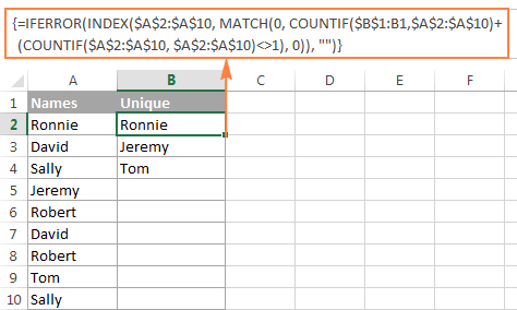
The detailed explanation of the formula's logic is provided in a separate section, and here's how to use the formula to extract unique values in your Excel worksheets:
- Tweak one of the formulas according to your dataset.
- Enter the formula in the first cell of the unique list (B2 in this example).
- If you are using the array formula, press Ctrl + Shift + Enter. If you've opted for the regular formula, press the Enter key as usual.
- Copy the formula down as far as needed by dragging the fill handle. Since both unique values formulas are we encapsulated in the IFERROR function, you can copy the formula up to the end of your table, and it won't clutter your data with any errors no matter how few unique values have been extracted.
How to get distinct values in Excel (unique + 1st duplicate occurrences)
As you may have already guessed from the heading of this section, distinct values in Excel are all different values in a list, i.e. unique values and first instances of duplicate values. For example:

To get a distinct list in Excel, use the following formulas.
Array distinct formula (requires pressing Ctrl + Shift + Enter):
=IFERROR(INDEX($A$2:$A$10, MATCH(0, COUNTIF($B$1:B1, $A$2:$A$10), 0)), "")
Regular distinct formula:
=IFERROR(INDEX($A$2:$A$10, MATCH(0, INDEX(COUNTIF($B$1:B1, $A$2:$A$10), 0, 0), 0)), "")
Where:
- A2:A10 is the source list.
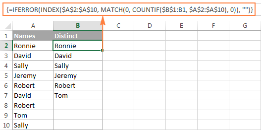
- B1 is the cell above the first cell of the distinct list. In this example, the distinct list begins in cell B2 (it's the first cell where you enter the formula), so you reference B1.
Extract distinct values in a column ignoring blank cells
If your source list contains any blank cells, the distinct formula we've just discussed would return a zero for each empty row, which might be a problem. To fix this, improve the formula a bit further:
Array formula to extract distinct values excluding blanks:
=IFERROR(INDEX($A$2:$A$10, MATCH(0, COUNTIF($B$1:B1, $A$2:$A$10&"") + IF($A$2:$A$10="",1,0), 0)), "")
Get a list of distinct text values ignoring numbers and blanks
In a similar manner, you can get a list of distinct values excluding empty cells and cells with numbers:
=IFERROR(INDEX($A$2:$A$10, MATCH(0, COUNTIF($B$1:B1, $A$2:$A$10&"") + IF(ISTEXT($A$2:$A$10)=FALSE,1,0), 0)), "")
As a quick reminder, in the above formulas, A2:A10 is the source list, and B1 is cell right above the first cell of the distinct list.
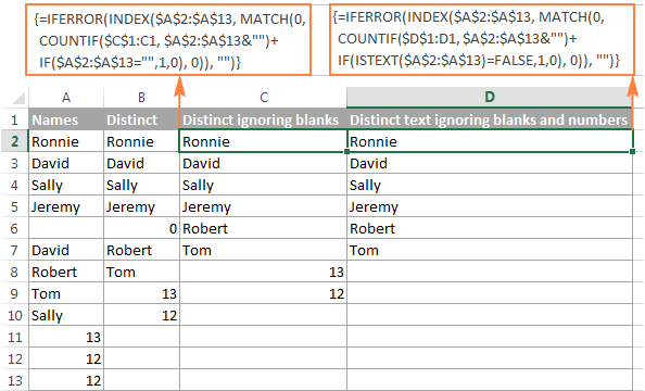
The following screenshot shows the result of both formulas:
How to extract case-sensitive distinct values in Excel
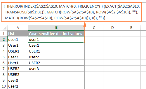
When working with case-sensitive data such as passwords, user names or file names, you may need to get a list of case-sensitive distinct values. For this, use the following array formula, where A2:A10 is the source list, and B1 is the cell above the first cell of the distinct list:
Array formula to get case-sensitive distinct values (requires pressing Ctrl + Shift + Enter)
=IFERROR(INDEX($A$2:$A$10, MATCH(0, FREQUENCY(IF(EXACT($A$2:$A$10,TRANSPOSE($B$1:B1)), MATCH(ROW($A$2:$A$10), ROW($A$2:$A$10)), ""), MATCH(ROW($A$2:$A$10), ROW($A$2:$A$10))), 0)), "")
How the unique / distinct formula works
This section is written especially for those curious and thoughtful Excel users who not only want to know the formula but fully understand its nuts and bolts.
It goes without saying that the formulas to extract unique and distinct values in Excel are neither trivial nor straightforward. But having a closer look, you may notice that all the formulas are based on the same approach - using INDEX/MATCH in combination with COUNTIF, or COUNTIF + IF functions.
For our in-depth analysis, let's use the array formula that extracts a list of distinct values because all other formulas discussed in this tutorial are improvements or variations of this basic one:
=IFERROR(INDEX($A$2:$A$10, MATCH(0, COUNTIF($B$1:B1, $A$2:$A$10), 0)), "")

For starters, let's cast away the obvious IFERROR function, which is used with a single purpose to eliminate #N/A errors when the number of cells where you've copied the formula exceeds the number of distinct values in the source list.
And now, let's break down the core part of our distinct formula:
- COUNTIF(range, criteria) returns the number of cells within a range that meet a specified condition.
In this example, COUNTIF($B$1:B1, $A$2:$A$10) returns an array of 1's and 0's based on whether any of the values of the source list ($A$2:$A$10) appears somewhere in the distinct list ($B$1:B1). If the value is found, the formula returns 1, otherwise - 0.
In particular, in cell B2, COUNTIF($B$1:B1, $A$2:$A$10) becomes:
COUNTIF("Distinct", {"Ronnie"; "David"; "Sally"; "Jeremy"; "Robert"; "David"; "Robert"; "Tom"; "Sally"})and returns:
{0;0;0;0;0;0;0;0;0}because none of the items of the source list (criteria) appears in the range where the function looks for a match. In this case, range ($B$1:B1) consists of a single item - "Distinct".
MATCH(lookup_value, lookup_array, [match_type])returns the relative position of the lookup value in the array.
In this example, the lookup_value is 0, and consequently:MATCH(0,COUNTIF($B$1:B1, $A$2:$A$10), 0)turns into:
MATCH(0, {0;0;0;0;0;0;0;0;0},0)and returns 1
because our MATCH function gets the first value that is exactly equal to the lookup value (as you remember, the lookup value is 0).
- INDEX(array, row_num, [column_num]) returns a value in an array based on the specified row and (optionally) column numbers.
In this example, INDEX($A$2:$A$10, 1)
becomes:
INDEX({"Ronnie"; "David"; "Sally"; "Jeremy"; "Robert"; "David"; "Robert"; "Tom"; "Sally"}, 1)and returns "Ronnie".
When the formula is copied down the column, the distinct list ($B$1:B1) expands because the second cell reference (B1) is a relative reference that changes according to the relative position of the cell where the formula moves.
So, when copied to cell B3, COUNTIF($B$1:B1, $A$2:$A$10) changes to COUNTIF($B$1:B2, $A$2:$A$10), and becomes:
COUNTIF({"Distinct";"Ronnie"}, {"Ronnie"; "David"; "Sally"; "Jeremy"; "Robert"; "David"; "Robert"; "Tom"; "Sally"}), 0)), "")and returns:
{1;0;0;0;0;0;0;0;0}because one "Ronnie" is found in range $B$1:B2.
And then, MATCH(0,{1;0;0;0;0;0;0;0;0},0) returns 2, because 2 is the relative position of the first 0 in the array.
And finally,
INDEX($A$2:$A$10, 2)returns the value from the 2nd row, which is "David".
Tip. For better understanding of the formula's logic, you can select different parts of the formula in the formula bar and press F9 to see what a selected part evaluates to:

If you still have difficulties figuring out the formula, you can check out the following tutorial for the detailed explanation of how the INDEX/MATCH liaison works: INDEX & MATCH as a better alternative to Excel VLOOKUP.
As already mentioned, the other formulas discussed in this tutorial are based on the same logic, with just a few modifications:
Unique values formula - contains one more COUNTIF function that excludes from the unique list all items that appear in the source list more than once: COUNTIF($A$2:$A$10, $A$2:$A$10)<>1.
Distinct values formula ignoring blanks - here you add an IF function that prevents blank cells from being added to the distinct list: IF($A$2:$A$13="",1,0).
Distinct text values formula ignoring numbers - you use the ISTEXT function to check whether a value is text, and the IF function to dismiss all other value types, including blank cells: IF(ISTEXT($A$2:$A$13)=FALSE,1,0).
Extract distinct values from a column with Excel's Advanced Filter
If you don't want to waste time on figuring out the arcane twists of the distinct value formulas, you can quickly get a list of distinct values by using the Advanced Filter. The detailed steps follow below.
- Select the column of data from which you want to extract distinct values.
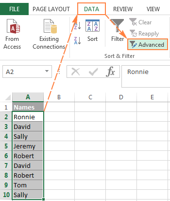
- Switch to the Data tab > Sort & Filter group, and click the Advanced button:
- In the Advanced Filter dialog box, select the following options:
- Check Copy to another location radio button.
- In the List range box, verify that the source range is displayed correctly.
- In the Copy to box, enter the topmost cell of the destination range. Please keep in mind that you can copy the filtered data only to the active sheet.
- Select the Unique records only

- Finally, click the OK button and check the result:

Please pay attention that although the Advanced Filter's option is named "Unique records only", it extracts distinct values, i.e. unique values and 1st occurrences of duplicate values.
Extract unique and distinct rows with Duplicate Remover
In the final part of this tutorial, let me show you our own solution to find and extract distinct and unique values in Excel sheets. This solution combines the versatility of Excel formulas and simplicity of the advanced filter. In addition, it provides a couple of unique features such as:
- Find and extract unique / distinct rows based on values in one or more columns.
- Find, highlight, and copy unique values to any other location, in the same or different workbook.
And now, let's see the Duplicate Remover tool in action.
Supposing you have a summary table created by consolidating data from several other tables. Obviously, that summary table contains a lot of duplicate rows and your task is to extract unique rows that appear in the table only once, or distinct rows including unique and 1st duplicate occurrences. Either way, with the Duplicate Remover add-in the job is done in 5 quick steps.
- Select any cell within your source table and click the Duplicate Remover button on the Ablebits Data tab, in the Dedupe group.

The Duplicate Remover wizard will run and select the entire table. So, just click Next to proceed to the next step.

- Select the value type you want to find, and click Next:
- Unique
- Unique +1st occurrences (distinct)
In this example, we aim to extract unique rows that appear in the source table only once, so we select the Unique option:

Tip. As you can see in the above screenshot, there are also 2 options for duplicate values, just keep it in mind if you need to dedupe some other worksheet.
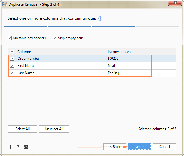
- Select one or more columns to be checked for unique values.
In this example, we want to find unique rows based on values in all 3 columns (Order number, First name and Last name), therefore we select all.
- Choose the action to perform on the found unique values. The following options are available to you:
- Highlight unique values
- Select unique values
- Identify in a status column
- Copy to another location
Because we are extracting unique rows, select Copy to another location, and then specify where exactly you want to copy them - active sheet (select the Custom location option, and specify the top cell of the destination range), new worksheet or new workbook.
In this example, let's opt for the new sheet:

- Click the Finish button, and you are done!

Liked this quick and simple way to get a list of unique values or rows in Excel? If so, I encourage you to download an evaluation version below and give it a try. Duplicate Remover as well as all other time-saving tools that we have are included with Ultimate Suite for Excel.
Available downloads
Find Unique Values in Excel - sample workbook (.xlsx file)
Ultimate Suite - evaluation version (.exe file)
 by
by
75 comments
Hi,
Please suggest a formula to get distinct texts from Column C and add totals against that text from Column B while matching the criteria in Column A. Here is an example:
A1 A B C
2 AA 1000 Closed
3 AA 250 Closed
4 AA 100 Partially Closed
5 AA 400 Open
6 AA 150 Open
7 AA 800 Partially Closed
8 AB 900 Done
9 AB 500 Pending
10 AB 450 Partially Done
11 AB 200 No update
12 AB 350 Partially Done
13 AB 650 Pending
14 AB 700 Done
15 AB 200 Partially Done
I need the entire text in one cell against each item in Column A:
AA: "1250: Closed
900: Partially Closed
550: Open"
AB: "1600: Done
1150: Pending
1000: Partially Done
200: No Update"
Here is the formula that I tried in Column H : =TEXTJOIN(CHAR(10),TRUE,TEXT(SUMIFS($C$2:$C$15,$B$2:$B$15,$G2,$D$2:$D$15,IFERROR(INDEX($D$2:$D$15,MATCH(0,IF((($B$2:$B$15=$G2)),COUNTIF($H$1:H1,$D$2:$D$15),""),0)),"")),"$#,##0_);($#,##0)"),"")&": "&IFERROR(INDEX($D$2:$D$15,MATCH(0,IF((($B$2:$B$15=$G2)),COUNTIF($H$1:H1,$D$2:$D$15),""),0)),"")
However, it's returning the text as mentioned below in Column H i.e only the 1st distinct text along with the sum against that text.
G H
AA $1,250 : Closed
Would greatly appreciate your help.
Thank you!
Hi! Your problem cannot be solved with a single formula. You can get a list of unique values in two columns using the UNIQUE function, and then in the third column use the SUMIFS function to calculate the sum of the two conditions in each row.
For the regular distinct formula there is an additional Index function with row and column = 0.
This does not appear in the array formula.
Could you please explain what the purpose of this index function is and why it is necessary?
When I remove this from the formula it no longer works.
Regular distinct formula:
=IFERROR(INDEX($A$2:$A$10, MATCH(0, INDEX(COUNTIF($B$1:B1, $A$2:$A$10), 0, 0), 0)), "")
Thanks,
Hi! Formula INDEX(COUNTIF($B$1:B1, $A$2:$A$10), 0, 0) is used instead of a formula COUNTIF($B$1:B1, $A$2:$A$10) to avoid entering it as an array formula using Ctrl + Shift + Enter.
How to count distinct value in a row ?
For e.g
Column1 Column2 Column3 Column4 Count of Distinct country
USA INDIA UK UK 3
USA USA USA USA 0
UK FRANCE UAE PERU 4
Hello!
You can find the examples and detailed instructions here: Count unique and distinct values in Excel with formula or pivot table.
Thank you Svetlana and all others commenting on this excel topic. May I ask how functions would differ if we were attempting to do the same with multiple rows?
In the example above for ignoring blanks, but allowing for numbers. I modified the table to include original Names column and added Names2. I'm allowing for numbers since my dataset/table has numbers. The function I thought would work is as follows:
=IFERROR(INDEX($A$2:$B$14,MATCH(0, COUNTIF($D$1:D5,$A$2:$B$14&"")+IF($A$2:$B$14="",1,0),0)),"")
Columns A and B are Names and Names2 respectively. How would I go about doing multiple columns? What if columns weren't side-by-side?
Thank you ahead of time. AZ
Hello!
Here is a formula that will find all distinct values (text and numbers) in two columns A and B ignoring blanks. Write it in D2 and copy it down the column.
=IFERROR(IFERROR(INDEX($A$2:$A$20, MATCH(0,COUNTIF($D$1:D1,$A$2:$A$20)+($A$2:$A$20=""),0)), INDEX($B$2:$B$20, MATCH(0,COUNTIF($D$1:D1,$B$2:$B$20)+($B$2:$B$20=""),0))),"")
I hope my advice will help you solve your task.
Perhaps I declared victory too soon. I was hoping to extrapolate from the "2 column" example of acquiring unique values to go from 2 to 3 to 4 and so on and so forth, but running into some difficulties that perhaps you can assist with.
To recap, and this is more for my understanding since I'm a getting all tangled up with this not so intuitive excel function. We started with one column which seemed to work.
=IFERROR(
INDEX($A$2:$B$14,MATCH(0, COUNTIF($D$1:D5,$A$2:$B$14&"")+IF($A$2:$B$14="",1,0),0)),"")
The two column function was as follows:
=IFERROR(IFERROR(
INDEX($A$2:$A$20, MATCH(0,COUNTIF($D$1:D1,$A$2:$A$20)+($A$2:$A$20=""),0)),
INDEX($B$2:$B$20, MATCH(0,COUNTIF($D$1:D1,$B$2:$B$20)+($B$2:$B$20=""),0))),"")
Moving on to three columns is failing and not sure why. What am I doing wrong?
=IFERROR(IFERROR(IFERROR(
INDEX($A$2:$A$20, MATCH(0,COUNTIF($D$1:D1,$A$2:$A$20)+($A$2:$A$20=""),0)),
INDEX($B$2:$B$20, MATCH(0,COUNTIF($D$1:D1,$B$2:$B$20)+($B$2:$B$20=""),0)),
INDEX($C$2:$C$20, MATCH(0,COUNTIF($D$1:D1,$C$2:$C$20)+($C$2:$C$20=""),0))
)),"")
I'm adding white space for better visualization. Thanks for the help.
Hello!
Here is an array formula that finds distinct values in three columns –
=IFERROR(IFERROR(IFERROR(INDEX($A$2:$A$20,MATCH(0,COUNTIF($D$1:D1,$A$2:$A$20)+($A$2:$A$20=""),0)), INDEX($B$2:$B$20,MATCH(0,COUNTIF($D$1:D1,$B$2:$B$20)+($B$2:$B$20=""),0))), INDEX($C$2:$C$20,MATCH(0,COUNTIF($D$1:D1,$C$2:$C$20)+($C$2:$C$20=""),0))),"")
Hope this is what you need.
Thanks Alexander!
That seems to have worked. A step closer to counting unique values from multiple columns. As I count additional columns I'll keep increasing the function. By the time all is said and done I'll have over 100 columns to count. A tad bit primitive but It's a solution for the meantime until I transition to another development environment such as Python.
Thanks for the help!
multiple columns... not rows. My apologies.
How would I get a unique minimum value in row F
R0 A B C D E Unique Minimum
R1 1 2 3 4 5 1
R2 2 3 4 5 6 2
R3 2 3 6 8 9 3 - because 2 is already in place in R2
Over 1 thousand rows to check
Hi!
You can solve your problem with a VBA macro.
Small update to my question
I am trying just something very simple as table:
Just 2 columns: Names | UNIQUE
In the column Names we have "texts" as below
00340312891320582291
00340312891920067756
00340312891920069262
00340312891320580598
00340312891320578410
00340312891320578189
00340312891320578854
00340312891320577890
00340312891320578231
00340312891320577661
In the column UNIQUE - should appear only unique values, in this example everything is unique but to compare it it must be as text not numbers like all the time.
Ignore please concatenate in my message before, its just trying to find a way. I clearly use your description and it not works for this example - only when I add prefix as letter or something :(
Help please - from one column to another just unique, especially if it can works with Table - area defined as table
Thanks,
Dawid
Hello!
If I understand correctly, you want to keep leading zeros in numbers. An easy way to preserve leading zeros in Excel is to precede the number with an apostrophe ('). For example, instead of entering 0034, enter '0034.
Without this, Excel will ignore leading zeros and will convert your text to a number.
The following tutorial should help: How to keep leading zeros in Excel.
Great teaching. Thanks.
I’d like to get the unique alphabetically sorted.
Using Excel 365’s SORT function in various places in the first formula you show, I can’t get SORT to do anything.
Is that because the SORT function has to happen after the list is extracted, and there is no way to set the order of the functions?
Thanks.
Hello!
Maybe this instructions will help you: Sort and filter in Excel or Excel unique values sorted alphabetically.
Regarding trying to use the SORT function combined with the unique lost process:
I tried just a manual Sort on the unique column, but nothing seemed to happen. It’s possible it did soft the formula cells but it returned with the same list, first found-last found. Probably because it is going back to the data and finding it again in the same order.
FILTER function wouldn’t help with this unique formula as there is nothing to filter until it is all done. (I assume.)
So, I could sort the source data. But will just continue with a helped column where the SORT function sorts the unique list. Easier since it is now programmed in, no macros needed.
IN my case I've got a sheet containing a list of appointments between sales people and clients, and I'm trying to count the number of clients each sales person has. To this end, I've used your list distinct values formula to create a list in a column of each sales person, but in a row beside those, I'm trying to create a horizontal list of all distinct clients that sales person has seen. How would I adapt the formula to generate that list of clients?
Thanks for any help!
Hello!
You can find the examples and detailed instructions here: Get a list of unique values based on criteria.
To write the result in one cell, you can use the TEXTJOIN function:
=TEXTJOIN(", ",TRUE,UNIQUE(FILTER(A2:A10,C2:C10=F1),FALSE))
I hope I answered your question. If something is still unclear, please feel free to ask.
Hi
Many thanks for this article. I have data like the below in sheet TZ. In another sheet, I am listing the unique dates under column J.
Date | Amount | CODE
(column B)
------- ----------- ---------
15-JUL-2021 25000 HIN
15-JUL-2021 22000 HIN
13-JUL-2021 42000 TIN
12-JUL-2021 37000 HIN
07-JUL-2021 26000 PIN
06-JUL-2021 14000 HIN
From this list, I want to extract distinct values of date corresponding to a code HIN alone.
Can you please help with this?
=IFERROR(INDEX(TZ!$B$2:TZ!$B$1746, MATCH(0, IF(ISBLANK(TZ!$B$2:TZ!$B$1746),1,COUNTIFS($J$1:J1, TZ!$B$2:TZ!$B$1746) ), 0)), "")
Hello!
You can find the examples and detailed instructions here: Get a list of unique values based on criteria.
I hope it’ll be helpful. If something is still unclear, please feel free to ask.
Hi
I have a list of historical orders as follows
Harry Skirt1
Harry Skirt2
Harry Skirt2
Harry Tie1
Harry Tie1
Harry Skirt1
Tony Trouser1
Tony Skirt1
Tony Trouser1
Tony Skirt1
What I want to be able to do is type customer name into a box and list the products they took (removing duplications)
So in a cell I type (or choose from a list) Harry
That gives me:
Skirt1
Skirt2
Tie1
How do I do that - I have a lot of data as its listed by SKU (style / colour / size) so the formula in the instructions took a long time to load up
Appreciate any help guys
Hello!
You can find the examples and detailed instructions here: Get a list of unique values based on criteria.
I hope my advice will help you solve your task.
Hi,
How do I modify the formula below if I have another criteria column:
=IFERROR(INDEX($A$8:$A$8, MATCH(0, INDEX(COUNTIF($C$1:C1, $A$2:$A$8), 0, 0), 0)), "")
For example:
A1 B1
Pete C
Betty C
Frank C
Mary O
Frank O
Mary O
Suzy O
I want the formula to look only at rows with "O" and return distinct names.
Result:
C1
Mary
Frank
Suzy
Your help is much appreciated! Thank you!
Hello!
If I got you right, the formula below will help you with your task:
=IFERROR(INDEX(FILTER(A2:A10,B2:B10="O"), MATCH(0, COUNTIF($C$1:C1, FILTER(A2:A10,B2:B10="O")), 0)), "")
This is an array formula and it needs to be entered via Ctrl + Shift + Enter, not just Enter.
Hi,
How to How to get distinct values in Excel (unique + 1st duplicate occurrences), based in a cell reference
for example
Column A Column B
A Apple
B Banana
A pineapple
C Orange
A Apple
I want a list of distinct values based in column A i.e if A, then
Apple
Pine Apple
if B
Banana
Help Please, Thanks in advance
Hello!
Study the section in this article, "How to get distinct values in Excel." If you have specific questions after that, I will try to answer them.
Hi
I am trying to do a lookup from one sheet within multiple rows and columns.
Customer, Part number will have different qty breaks with different prices.
Rows have duplicate part numbers and customer, possible price.
Thanks
How would you recommend the easiest way?
I'd recommend you to have a look at our Ablebits Data - Vlookup Wizard. This tool is available as a part of our Ultimate Suite for Excel that you can install in a trial mode and use for 30 days for free: https://www.ablebits.com/files/get.php?addin=xl-suite&f=free-trial
I have two sheets
First sheet has 470 records, some duplicates.
Second sheet has 1000 records, some duplicates.
I want to find all unique values on sheet one that are NOT on sheet two.
So, any value found in sheet two that matches on sheet one will not be shown. I only want unique values from sheet one. If there are duplicates within sheet one that are not on sheet two they should remain after filtering.
Hello!
You want to find duplicates twice. Using one formula is not possible. I recommend using Duplicate Remover. This tool is available as a part of our Ultimate Suite for Excel that you can install in a trial mode and use for free: https://www.ablebits.com/files/get.php?addin=xl-suite&f=free-trial
Can I get a formula to remove duplicates and blanks when the data is displayed in a row. I tried to make some changes in the formula which is mentioned for data placed in a column, but couldn't get the desired results.
Hello Keshav!
If the list of values is on the line (for example, A2:P2), then the list of unique values can be obtained using the formula in cell S2.
Regular unique values formula (completed by pressing Enter):
=IFERROR(INDEX($A$2:$P$2, MATCH(0,INDEX(COUNTIF($S$1:S1, $A$2:$P$2) + (COUNTIF($A$2:$P$2, $A$2:$P$2)<>1),0,0), 0)), "")
In cell U2, we write the formula of the array (completed by pressing Ctrl + Shift + Enter):
=IFERROR(INDEX($A$2:$P$2, MATCH(0, COUNTIF($U$1:U1,$A$2:$P$2) + (COUNTIF($A$2:$P$2, $A$2:$P$2)<>1), 0)), "")
After that you can copy this formula down along the column.
Regarding the formula +IFERROR(INDEX($A$2:$A$10, MATCH(0, COUNTIF($B$1:B1, $A$2:$A$10), 0)), ""), I only getting the first value as it takes B1 and does not update to b2 b3 and so on when I use it. The array is not working.
Hello,
You write this formula in cell B2.This is an array formula and it needs to be entered via Ctrl + Shift + Enter, not just Enter. You have not done so. After that you can copy this formula down along the column.
=IFERROR(INDEX($A$2:$A$10, MATCH(0, INDEX(COUNTIF($B$1:B1, $A$2:$A$10), 0, 0), 0)), "") works but one needs to figure out how many distinct values are going to exist in order to copy and paste the formula that many times. Hence, if there are 10 distinct values then one copies and paste the formula 9 times. Is there a way for one does not need to know how many distinct values are going to exist?
Thank you
Hello!
To calculate the number of unique values in a data range, use the formula
=SUMPRODUCT(COUNTIF(A2:A20,A2:A20)^(2*ISBLANK(A2:A20)-1))
I hope this will help, otherwise please do not hesitate to contact me anytime.
I have a list of employees and each has a unique job category. Based on their job category, I want a unique list of job competencies to show up to select from a pull down list that are only available for that job category.
Hello!
Use cascading dropdown list
This link has detailed instructions on our blog.
If there is anything else I can help you with, please let me know.
how this part is working =COUNTIF($A$2:$A$10, $A$2:$A$10)
& how this is different from this =COUNTIF($A$2:$A$10,A2)1 since both has same result separately but in formula second option isn't working,please also explain this part more =COUNTIF($J$1:J1, $A$2:$A$10)...??thnx
this one is correct, =COUNTIF($A$2:$A$10,A2) wrongly place 1 at the end.
Hello,
I have two Worksheets---WS1 Customer column A(match)& Customer Number B(return value) ....WS2 Customer column E ...WS 2 Column Q (formula)- I need a formula that will match WS2 Column E to Column A WS1 and return value of column B WS1
Thank you in advance!!
To add the columns in WS 1 Customer are not alphabetized. So, therefore other index match formulas I am using, are not working.