The tutorial explains how to split cells in Excel using formulas and the Split Text feature. You will learn how to separate text by comma, space or any other delimiter, and how to split strings into text and numbers.
Splitting text from one cell into several cells is the task all Excel users are dealing with once in a while. In one of our earlier articles, we discussed how to split cells in Excel using the Text to Column feature and Flash Fill. Today, we are going to take an in-depth look at how you can split strings using formulas and the Split Text tool.
How to split text in Excel using formulas
To split string in Excel, you generally use the LEFT, RIGHT or MID function in combination with either FIND or SEARCH. At first sight, some of the formulas might look complex, but the logic is in fact quite simple, and the following examples will give you some clues.
Split string by comma, semicolon, slash, dash or other delimiter
When splitting cells in Excel, the key is to locate the position of the delimiter within the text string. Depending on your task, this can be done by using either case-insensitive SEARCH or case-sensitive FIND. Once you have the delimiter's position, use the RIGHT, LEFT or MID function to extract the corresponding part of the text string. For better understanding, let's consider the following example.
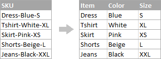
Supposing you have a list of SKUs of the Item-Color-Size pattern, and you want to split the column into 3 separate columns:
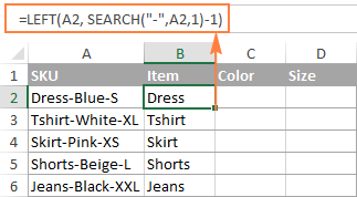
- To extract the item name (all characters before the 1st hyphen), insert the following formula in B2, and then copy it down the column:
=LEFT(A2, SEARCH("-",A2,1)-1)In this formula, SEARCH determines the position of the 1st hyphen ("-") in the string, and the LEFT function extracts all the characters left to it (you subtract 1 from the hyphen's position because you don't want to extract the hyphen itself).
- To extract the color (all characters between the 1st and 2nd hyphens), enter the following formula in C2, and then copy it down to other cells:
=MID(A2, SEARCH("-",A2) + 1, SEARCH("-",A2,SEARCH("-",A2)+1) - SEARCH("-",A2) - 1)
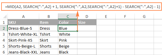
In this formula, we are using the Excel MID function to extract text from A2.
The starting position and the number of characters to be extracted are calculated with the help of 4 different SEARCH functions:
- Start number is the position of the first hyphen +1:
SEARCH("-",A2) + 1 - Number of characters to extract: the difference between the position of the 2nd hyphen and the 1st hyphen, minus 1:
SEARCH("-", A2, SEARCH("-",A2)+1) - SEARCH("-",A2) -1
- Start number is the position of the first hyphen +1:
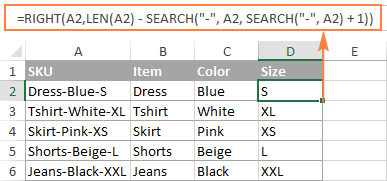
- To extract the size (all characters after the 3rd hyphen), enter the following formula in D2:
=RIGHT(A2,LEN(A2) - SEARCH("-", A2, SEARCH("-", A2) + 1))In this formula, the LEN function returns the total length of the string, from which you subtract the position of the 2nd hyphen. The difference is the number of characters after the 2nd hyphen, and the RIGHT function extracts them.
In a similar fashion, you can split column by any other character. All you have to do is to replace "-" with the required delimiter, for example space (" "), comma (","), slash ("/"), colon (";"), semicolon (";"), and so on.
Tip. In the above formulas, +1 and -1 correspond to the number of characters in the delimiter. In this example, it's a hyphen (1 character). If your delimiter consists of 2 characters, e.g. a comma and a space, then supply only the comma (",") to the SEARCH function, and use +2 and -2 instead of +1 and -1.
How to split string by line break in Excel
To split text by space, use formulas similar to the ones demonstrated in the previous example. The only difference is that you will need the CHAR function to supply the line break character since you cannot type it directly in the formula.
Supposing, the cells you want to split look similar to this:
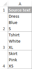
Take the formulas from the previous example and replace a hyphen ("-") with CHAR(10) where 10 is the ASCII code for Line feed.
- To extract the item name:
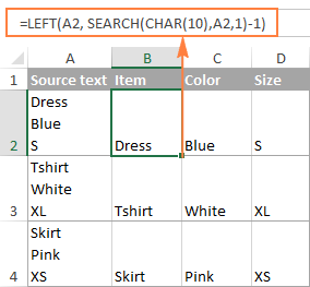
=LEFT(A2, SEARCH(CHAR(10),A2,1)-1) - To extract the color:
=MID(A2, SEARCH(CHAR(10),A2) + 1, SEARCH(CHAR(10),A2,SEARCH(CHAR(10),A2)+1) - SEARCH(CHAR(10),A2) - 1) - To extract the size:
=RIGHT(A2,LEN(A2) - SEARCH(CHAR(10), A2, SEARCH(CHAR(10), A2) + 1))
And this is how the result looks like:
How to split text and numbers in Excel
To begin with, there is no universal solution that would work for all alphanumeric strings. Which formula to use depends on the particular string pattern. Below you will find the formulas for the two common scenarios.
Split string of 'text + number' pattern
Supposing, you have a column of strings with text and numbers combined, where a number always follows text. You want to break the original strings so that the text and numbers appear in separate cells, like this:
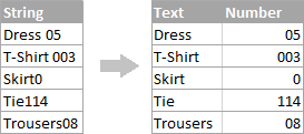
The result may be achieved in two different ways.
Method 1: Count digits and extract that many chars
The easiest way to split text string where number comes after text is this:
To extract numbers, you search the string for every possible number from 0 to 9, get the numbers total, and return that many characters from the end of the string.
With the original string in A2, the formula goes as follows:
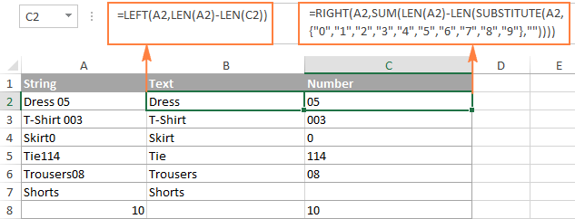
=RIGHT(A2,SUM(LEN(A2) - LEN(SUBSTITUTE(A2, {"0","1","2","3","4","5","6","7","8","9"},""))))
To extract text, you calculate how many text characters the string contains by subtracting the number of extracted digits (C2) from the total length of the original string in A2. After that, you use the LEFT function to return that many characters from the beginning of the string.
=LEFT(A2,LEN(A2)-LEN(C2))
Where A2 is the original string, and C2 is the extracted number, as shown in the screenshot:
Method 2: Find out the position of the 1st digit in a string
An alternative solution would be using the following formula to determine the position of the first digit in the string:
=MIN(SEARCH({0,1,2,3,4,5,6,7,8,9},A2&"0123456789"))
Once the position of the first digit is found, you can split text and numbers by using very simple LEFT and RIGHT formulas.
To extract text:
=LEFT(A2, B2-1)
To extract number:
=RIGHT(A2, LEN(A2)-B2+1)
Where A2 is the original string, and B2 is the position of the first number.
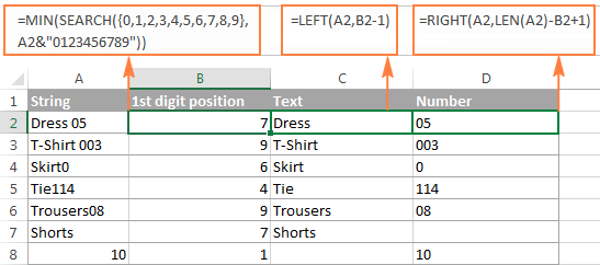
To get rid of the helper column holding the position of the first digit, you can embed the MIN formula into the LEFT and RIGHT functions:
Formula to extract text:
=LEFT(A2,MIN(SEARCH({0,1,2,3,4,5,6,7,8,9},A2&"0123456789"))-1)
Formula to extract numbers:
=RIGHT(A2,LEN(A2)-MIN(SEARCH({0,1,2,3,4,5,6,7,8,9},A2&"0123456789"))+1)
Split string of 'number + text' pattern
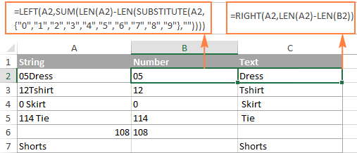
If you are splitting cells where text appears after number, you can extract numbers with the following formula:
=LEFT(A2, SUM(LEN(A2) - LEN(SUBSTITUTE(A2, {"0","1","2","3","4","5","6","7","8","9"}, ""))))
The formula is similar to the one discussed in the previous example, except that you use the LEFT function instead of RIGHT to get the number from the left side of the string.
Once you have the numbers, extract text by subtracting the number of digits from the total length of the original string:
=RIGHT(A2,LEN(A2)-LEN(B2))
Where A2 is the original string and B2 is the extracted number, as shown in the screenshot below:
Tip. To get number from any position in a text string, use either this formula or the Extract tool. Or you can create a custom function to split numbers and text into separate columns.
This is how you can split strings in Excel using different combinations of different functions. As you see, the formulas are far from obvious, so you may want to download the sample Excel Split Cells workbook to examine them closer.
If figuring out the arcane twists of Excel formulas is not your favorite occupation, you may like the visual method to split cells in Excel, which is demonstrated in the next part of this tutorial.
How to split cells in Excel with Split Text tool
An alternative way to split a column in Excel is using the Split Text feature included with our Ultimate Suite for Excel, which provides the following options:
To make things clearer, let's have a closer look at each option, one at a time.
Split cells by character
Choose this option whenever you want to split the cell contents at each occurrence of the specified character.
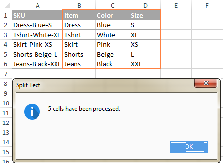
For this example, let's the take the strings of the Item-Color-Size pattern that we used in the first part of this tutorial. As you may remember, we separated them into 3 different columns using 3 different formulas. And here's how you can achieve the same result in 2 quick steps:
- Assuming you have Ultimate Suite installed, select the cells to split, and click the Split Text icon on the Ablebits Data tab.
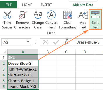
- The Split Text pane will open on the right side of your Excel window, and you do the following:
- Expand the Split by character group, and select one of the predefined delimiters or type any other character in the Custom box.
- Choose whether to split cells to columns or rows.
- Review the result under the Preview section, and click the Split button.
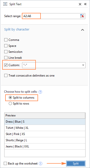
Tip. If there might be several successive delimiters in a cell (for example, more than one space character), select the Treat consecutive delimiters as one box.
Done! The task that required 3 formulas and 5 different functions now only takes a couple of seconds and a button click.
Split cells by string
This option lets you split strings using any combination of characters as a delimiter. Technically, you split a string into parts by using one or several different substrings as the boundaries of each part.
For example, to split a sentence by the conjunctions "and" and "or", expand the Split by strings group, and enter the delimiter strings, one per line:
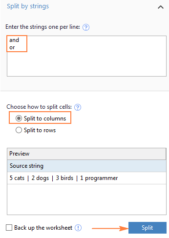
As the result, the source phrase is separated at each occurrence of each delimiter:

Tip. The characters "or" as well as "and" can often be part of words like "orange" or "Andalusia", so be sure to type a space before and after and and or to prevent splitting words.
And here another, real-life example. Supposing you've imported a column of dates from an external source, which look as follows:
5.1.2016 12:20
5.2.2016 14:50
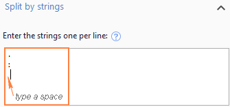
This format is not conventional for Excel, and therefore none of the Date functions would recognize any of the date or time elements. To split day, month, year, hours and minutes into separate cells, enter the following characters in the Split by strings box:
- Dot (.) to separate day, month, and year
- Colon (:) to separate hours and minutes
- Space to separate date and time
Hit the Split button, and you will immediately get the result:

Split cells by mask (pattern)
Separating a cell by mask means splitting a string based on a pattern.
This option comes in very handy when you need to split a list of homogeneous strings into some elements, or substrings. The complication is that the source text cannot be split at each occurrence of a given delimiter, only at some specific occurrence(s). The following example will make things easier to understand.
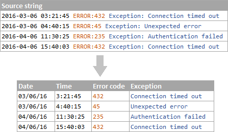
Supposing you have a list of strings extracted from some log file:

What you want is to have date and time, if any, error code and exception details in 3 separate columns. You cannot utilize a space as the delimiter because there are spaces between date and time, which should appear in one column, and there are spaces within the exception text, which should also appear in one column.
The solution is splitting a string by the following mask: *ERROR:*Exception:*
Where the asterisk (*) represents any number of characters.
The colons (:) are included in the delimiters because we don't want them to appear in the resulting cells.
And now, expand the Split by mask section on the Split Text pane, type the mask in the Enter delimiters box, and click Split:
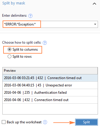
The result will look similar to this:

Note. Splitting string by mask is case-sensitive. So, be sure to type the characters in the mask exactly as they appear in the source strings.
A big advantage of this method is flexibility. For example, if all of the original strings have date and time values, and you want them to appear in different columns, use this mask:
* *ERROR:*Exception:*
Translated into plain English, the mask instructs the add-in to divide the original strings into 4 parts:
- All characters before the 1st space found within the string (date)
- Characters between the 1st space and the word ERROR: (time)
- Text between ERROR: and Exception: (error code)
- Everything that comes after Exception: (exception text)
I hope you liked this quick and straightforward way to split strings in Excel. If you are curious to give it a try, an evaluation version is available for download below. I thank you for reading and hope to see you on our blog next week!
Available downloads
Excel Split Cells formulas (.xlsx file)
Ultimate Suite 14-day fully-functional version (.exe file)
 by
by
308 comments
HOW can CONVERT this 0h1m2s to 00:01:02
Hi! Extract all numbers from the text as described in these instructions: Extract number from text string.
Using the formula below, insert a separator between these numbers and convert the text string to time using the TIMEVALUE function. For example:
=TIMEVALUE(SUBSTITUTE(TRIM(CONCAT(IF(ISNUMBER(--MID(H1,ROW($1:$20),1)),MID(H1,ROW($1:$20),1)," ")))," ",":"))
Set time format in the cell with the formula.
that's great
1. N0000000 - YUDHARSHAN
2. N0000000 - SARAF AHAMED SHAJAHAN
3. N0000000 - INDRARATHNA KASTHURI ARACHCHILAGE
4. N0000000 - SAMIRA PATHUM WICKRAMANAYAKA MUDALIGE
5. N0000000 - MOHAMMADH ASHAR ABDUL SAMADHU
6. N0000000 - LALITH PUSHPA KUMARA EDIRISINGHE EDIRISINGHE ARACHCHILAGE
7. EK000000 - XINHUAI LIN
8. N0000000 - MOHAMED ABDUR RAHEEM AHAMED LEBBE
9. N0000000 - NAFEER THOWFEEK
10. E0000000 - YIN JIE
This all in One Cell (A1). How can I split this into 3 columns and 10 Rows??
Hi! If I understand your task correctly, our Split Text tool may help you solve it in a few clicks. It allows you to split the text into rows and columns. To avoid blank rows or columns, you can treat several consecutive delimiters as one. It is available as a part of our Ultimate Suite for Excel that you can install in a trial mode and check how it works for free.
You can also try the TEXTSPLIT function to split the text. For example,
=TEXTSPLIT(A1,,CHAR(10))
Thanks so much! Saved me alot of time.
Hello, I'm looking to split the data below. Everything is in one column. Each row below is in once cell. The data information may change see below. Looking to separate each into its respective column. The number of spaces change per row. Appreciate your time and response with this matter. Have a bless day.
Row 1: RUN JAN 11 2023 HUNTINGTON PAGE 1
Row 2: SEQ# UNITS COST ACQUISITION COVERED HOW ACQUIRED MARKET VALUE OF GIFT DATE OF GIFT
Row 3: 41 27.0510 1,508.08 02/25/2021 C P
Row 4: POSTING DATE: 01/03/2023
Row 5: SECURITY ID: 01345678 BXXXXX TOTAL POSITION QUANTITY
Row 6: ---- --------- ---------- ------------- --------- ------------ -------------------- ------------
Row 7: JOHN W SMITH TOD AGENCY 123456789
Hello, I did try the TEXTSPLIT function. but it does not split the data. =TEXTSPLIT(A1, " "). Data is in (A1) I enter this =TEXTSPLIT(A1, " ") in AB and when I click enter nothing happens. In cell AB shows the formula entered. Do you recommend anything else? I would use the count spaces method but each row has multiple spaces in between each data. Appreciate your time and response.
Cell A1: SECURITY ID: 123456789 DAMIX TOTAL POSITION QUANTITY
Cell AB =TEXTSPLIT(A1, " ")
Hi! There is no other way to split text in Excel. The TEXTSPLIT function works in Excel365 and higher.
Hi! Have you tried the ways described in this blog post? If they don’t work for you, then try to use TEXTSPLIT function. Read more: TEXTSPLIT function in Excel: split text strings by delimiter.
I have a file that contains numbers and texts, one category has text that includes text with commas. I want to split my data into separate columns. When I used the "Text to Columns" tool, it also split the text that contains commas into different columns, how can I prevent that and only let it split the rest of the data?
Is there a way where I can download the file where the data is split already?
The same file I'm trying to download worked perfectly fine when I used my old laptop.
Hi!
If you are using Text to Columns tool, watch carefully which characters you use as separators in Step 2. To separate text by columns, you can use the methods described in the article above. You can also use the TEXTSPLIT function.
I'm trying to extract a selection from a string variable.( Ex. 1, 3, 4, 6, 13) I'd like to pull into a column if the example cell includes "3" put a 1, for yes, in a separate column. What I'm doing is also pulling out 13 because it includes the 3. Any suggestions?
Try using find instead.
=IFERROR(IF(FIND(" 3,",A1)>0,1,""),"")
A1 being the column with the values in it.
By searching for the whole "space 3 comma" you avoid numbers with a 3 in them. e.g 30, 13
The find returns the position it finds the value in, so the answer will be >0.
Not being in the string returns an #Value! error, which is why the iferror is there.
Hello!
Use the SEARCH function to find " 3" (with a space before the number).
Please use the formula below:
=--ISNUMBER(SEARCH(" 3",A1))
Hi
how can i split the values in once cell
we had a lots of ticket numbers on one cell, we are separating them using alt + enter
how can we split the values of one cell unto rows
ex. this values are written inside of one cell and separated using alt + enter
226703
226705
226710
226713
226714
Thanks!
Super easy version : use Text to columns, Delimited and untick all options and select other.
In the box for the character Hold down ALT and using numpad type 010. This is the line break code.
It should split your text with ease.
Assuming your values you listed in the example are in A1. In B1 you can use =VALUE(LEFT(A1,6)). in b2 to whichever column you need, put: =IFERROR(VALUE(MID($A$1,(7*(COLUMN()-2))+1,6)),""). Drag the formula across till you get them all appearing.
Saiph
Hello!
Because you have a lot of values in a cell that need to be separated, it's hard to use a formula. We have a ready-made solution for your task. I'd recommend you to have a look at our Split Text tool. It is available as a part of our Ultimate Suite for Excel that you can install in a trial mode and check how it works for free.
Hello, thank you for your article.
I am trying to split "Dress 05 Pants 02 Shirt 01" into "Dress 05" "Pants 02" "Shirt 01", either in horizontal or vertical in multiple cells/rows, with the purpose of counting how many separated strings there are (in this example: 3 strings).
Could you please help me with this?
Hello!
To count the number of separated strings, you can count the number of spaces in a cell using this formula:
=(LEN(A1)-LEN(SUBSTITUTE(A1," ",""))+1)/2
To split text into cells, try using the Excel Text to Columns feature.
Update: Please check out TEXTSPLIT, TEXTBEFORE, and TEXTAFTER functions to simplify practically everything mentioned in this article or the comments.
Hello!
These functions are currently available in Office Insider Beta only. However, you can read our blog:
TEXTSPLIT function in Excel: split cells / text strings by delimiter.
Excel TEXTBEFORE function - extract text before character (delimiter).
Excel TEXTAFTER function: extract text after character or word.
Hi,
I have a real problem that I can't find anything near what I need.
column (A) each cell has a single entry "CNN-001" which increments sequentially (CNN-002, CNN-003 etc).
column (B) has cells that can have a single entry "010001" or multiple entries using the 'Line Break' method (010001 alt+enter then 010002 alt+enter) etc. like a batch.
These numbers can repeat many times in column (B).
Column (C) has cells with a single entry "010001"
I want to do something like and Index and Match but it doesn't work with cells with multiple entries in it.
So I want to Index (A) and Match (C) to (B)
I can only use a formula and no macros.
Is this possible?
Any help will be greatly appreciated.
Thanks,
Mark.
Hello!
Use the SEARCH function to match two cells.
=ISNUMBER(SEARCH(C1,B1))
You can read different sorting methods in this article: Sort by row, by column names and in custom order.
I hope it’ll be helpful. If something is still unclear, please feel free to ask.
Hi Alexander,
Thank you for you're quick response.
I don't think I explained it as well as I thought I had, let me try again.
Workbook 1 : Source Data
Workbook 2 : Summary Document
(workbook 2 looks at Workbook 1 to find information)
(workbook 2 has a column (X) with a manually entered number e.g. "010001" per cell)
it will use "010001" to look in workbook 1 and find all "CNN" numbers in column (B) against "010001"
And list these "CNN" numbers in column (Z)
Workbook 1 column (A) : each cell can contain a single or multiple entry
e.g. 010001
or 010001 : this cell may contain up to 30-40 entries
010008
010010
Workbook 1 column (B) : each cell will contain just a single entry.
So, workbook 1 looks like this: Workbook 2 looks like this.
A B X Z ('Z' looks for 'X' in 'A' and reports 'B')
010001 CNN-001 010007 CNN-002
--------------------------------------- CNN-003
010007 ------------------------
010009 010021 CNN-004
010001 CNN-002 ------------------------
010003 010001 CNN-001
010036 CNN-002
-------------------------------- CNN-004
010007 CNN-003 ------------------------
--------------------------------
010019
010001 CNN-004
010021
--------------------------------
As you can see the numbers in 'A' are non-sequential and repeating.
I have found a work around where I can separate the numbers in 'A' into separate cells by adding more columns eg. (D,E,F,G etc) in wookbook 1 and using: -
(D) =TRIM(MID(SUBSTITUTE($A8,CHAR(10),REPT(" ",LEN($A8))),(D$7-1)*LEN($A8)+1,LEN($A8)))
(E) =TRIM(MID(SUBSTITUTE($A8,CHAR(10),REPT(" ",LEN($A8))),(E$7-1)*LEN($A8)+1,LEN($A8)))
(F) =TRIM(MID(SUBSTITUTE($A8,CHAR(10),REPT(" ",LEN($A8))),(F$7-1)*LEN($A8)+1,LEN($A8)))
etc.
I can then add new columns eg. (S,T,U,V,W) etc in workbook 2 and list all the column 'B' refereances against 'X' using: -
(S) =IFERROR(INDEX($B$8:$B$18,SMALL(IF($P8=$D$8:$M$18,ROW($D$8:$M$18)-ROW($D$8:$M$8)+1),ROW($1:$1))),"")
(T) =IFERROR(INDEX($B$8:$B$18,SMALL(IF($P8=$D$8:$M$18,ROW($D$8:$M$18)-ROW($D$8:$M$8)+1),ROW($2:$2))),"")
(U) =IFERROR(INDEX($B$8:$B$18,SMALL(IF($P8=$D$8:$M$18,ROW($D$8:$M$18)-ROW($D$8:$M$8)+1),ROW($3:$3))),"")
etc.
I then concatenate S,T,U,V & W into 'Z' and use line breaks using: -
=S8&CHAR(10)&T8&CHAR(10)&U8&CHAR(10)&V8&CHAR(10)&W8
It's not elegant and messy but I can't use any macros and I'm to dumb to work out a single formular to aichieve the same result.
Again,
Any help would be great.
Thanks,
Mark.
Hello!
If I understand your task correctly, try to get a list of the desired values using the FILTER function. You can merge these values in one cell using the TEXTJOIN function.
=TEXTJOIN(" ",TRUE,FILTER(A1:A5,ISNUMBER(SEARCH(C1,B1:B5))))
I hope it’ll be helpful.
Sorry I was trying to show what "workbook 1 and workbook 2 look like" but the spacing has all be changed so ignore that bit.
Mark.
Hello!
My goal is to split the text in a single cell into multiple cells
The single cell contains a product's brand and name:
Ex: "Brand Name Product Name Product Attributes"
I tried using a list of brand names as the delimiter in 'split text by substring' but ran into issues due to overlapping. "Nano" in the brand name can appear in the product name of other brands. Is there a best practice for separating brand & product information into multiple columns?
Thank you for your help!
Hello!
If your text has a common pattern, then it can be divided into cells. You may be able to use regular expressions to extract and split text.
Hi,
Could you please share how could I split mashed two emails addresses?
"example@company.comsecondexample@company.com"
Would there be a solution also if there were more emails smashed together?
Hello!
Use substring functions to split text:
=LEFT(A1,SEARCH(".com",A1)+3)
=MID(A1,SEARCH(".com",A1)+4,50)
Hello, this is so helpful thanks.
I do need help on how to separate this to display what is on the right.
Anna Clarence - 078933 Marcus Stuart - 05674 ==> Anna Clarence - 078933
==> Marcus Stuart - 05674
Patrick Wine - 0845 Oscar Lutherwood - 06522 ==> Patrick Wine - 0845
==>Lutherwood - 06522
Thanks!
Hi!
To split text on the fourth space, you can use the formulas:
=LEFT(A1,SEARCH("#",SUBSTITUTE(A1," ","#",4),1)-1)
=MID(A1,SEARCH("#",SUBSTITUTE(A1," ","#",4),1)+1,50)
I hope I answered your question.
I have a requirement to split one column data(say Column E) separated by ". "(dot and space) into new rows depends on quantity given in next column (say Column F). Also i need the same cell content of the splitted row for the all newly created Rows.
Input format :
CAPACITOR (in Column D) --> C1. C2.(in column E) --> 2 (in column F --> Kemet (in column G)
Expected result:
CAPACITOR (in Column D) --> C1(in column E) --> 2 (in column F --> Kemet (in column G)
CAPACITOR (in Column D) --> C2(in column E) --> 2 (in column F --> Kemet (in column G)
Thanks for the support
There is never a solution to split a text string with 4 sections into 4 seperate columns. I cannot use a text to columns approach either. I must take a string of data (1234567>xx-093456>DesignedBy>Weller&Sons). This information must be split into 4 separate columns on the worksheet. I can figure out how to use LEFT and MiD but the RIGHT never works. I cannot find a solution to break out the "Weller&Sons" no matter how hard I try. This is I am sure very simple for smarter excel users - but for me, I am manually typing hundreds of records a day, when I am certain there must be a trick that is not published. Seems most splits are with text to columns (I cannot use) and only for names (first and last). So, is there a solution out there that has not yet be developed or published, or is this an impossible task that will require me to carry on with the retyping of that last data point. Each day there are 100 more records to export and add details for. Thanks for any suggestions and aid.
Hello!
The most simple and convenient option for your task is Text to columns. If you can't use it, extract each word individually with these guidelines: How to extract Nth word from a text string.
You can also use the formula-free Ablebits Text Toolkit. It separates text into columns perfectly and contains many more options. Even more features are provided by Ablebits Ultimate Suite for Excel.
I hope I answered your question. If you have any other questions, please don’t hesitate to ask.
Good Day,
How to seperate this
METS$P0072;;HVA0302221;1;03/02/2022;03/02/2023;1;20.0
ITEM CODE BATCH MFG DATE EXP DATE QTY KILO
P0072 HVA0302221 03/02/2022 03/02/2023 1 20
THANK YOU VERY MUCH
Hello!
Have you tried the ways described in this blog post? Please re-check the article above since it covers your task.
Sorry I tried many times but failed to do so. I am asking for your help. This will be a great help for my report.
METS$P0072;;HVA0302221;1;03/02/2022;03/02/2023;1;20.0
This will be split into this
ITEM CODE
P0072
BATCH
HVA0302221
MFG DATE
03/02/2022
EXP DATE
03/02/2023
QTY
1
KILO
20
THANK YOU VERY MUCH.LOOKNIG FORWARD HEARING YOU SOON
Hi!
You can split text into cells using the Text to Columns tool.
To divide the first value you can use the formula -
=MID(A1,SEARCH("$",A1)+1,20)
Thank you very much <3
Hello,
I have a text string which i'd like to split by character at either "K" or "L". I've got the basic formula to split at one character, but I can't work out how to look for either a K or an L and then split the text there.
This is the formula I am using: =RIGHT(G13,LEN(G13)-FIND("K",G13))
These are examples of the text:
MC - K07.01
Suite I Water Inorganics Etc - L03.17
Hello!
If I understand your task correctly, the following formula should work for you:
=RIGHT(G13,LEN(G13)- (IFERROR(FIND("K",G13),1)*IFERROR(FIND("L",G13),1)))
I hope it’ll be helpful.
Thank you Alexander, that works well! I am also trying to retain the "K" or "L", is that something which is possible?
Hi!
Add 1 to the number of characters that the RIGHT function extracts
=RIGHT(G13,LEN(G13)- (IFERROR(FIND("K",G13),1)*IFERROR(FIND("L",G13),1))+1)
** The text I am looking to split would be like this:
MC - K07.01 to split "K07.01"
Etc - L03.17 to split "L03.17"
I have below alpha numeric line in A1 cell. I need sum of numeric from from space 27 i.e. 276 to /ON. Can you pls help?
XX¥XXXX111111/ .00/ 276.00/ 79.25/D43.38/D3.49/ON
I need to separate a string into 3 parts: 1-2 Prefix letters, number(1-3 digits) and a suffix letter. Every string may contain 1-4 characters, either just numbers or 1-3 of them.
String Example and the thing I want it to spit out:
2 (0,2,0)
2A (0,2,A)
46 (0,46,0)
60X (0,60,X)
208 (0,208,0)
234X (0,234,X)
H2 (H,2,0)
H1A (H,1,A)
A20 (A,20,0)
E21A (E,21,A)
X970 (X,970,0)
NA20 (NA,20,0)
(there is no 2 letter prefix+1 digit number+1 suffix in the strings)