In this tutorial, you will learn how to filter data in Excel in different ways: how to create filters for text values, numbers and dates, how to use filter with search, and how to filter by color or by selected cell's value. You will also learn how to remove filters, and how to fix Excel AutoFilter not working.
If working with large data sets, it can be a challenge not only to calculate data, but also to find the relevant information. Luckily, Microsoft Excel makes it easy for you to narrow down the search with a simple yet powerful Filter tool. To learn more about filtering in Excel, please click on the links below.
What is filter in Excel?
Excel Filter, aka AutoFilter, is a quick way to display only the information relevant at a given time and remove all other data from view. You can filter rows in Excel worksheets by value, by format and by criteria. After applying a filter, you can copy, edit, chart or print only visible rows without rearranging the entire list.
Excel Filter vs. Excel Sort
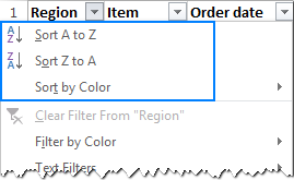
Apart from numerous filtering options, Excel AutoFilter provides the Sort options relevant to a given column:
- For text values: Sort A to Z, Sort Z to A, and Sort by Color.
- For numbers: Sort Smallest to Largest, Sort Largest to Smallest, and Sort by Color.
- For dates: Sort Oldest to Newest, Sort Newest to Oldest, and Sort by Color.
The difference between sorting and filtering in Excel is as follows:
- When you sort data in Excel, the entire table is rearranged, for example alphabetically or from the lowest to the highest value. However, sorting does not hide any entries, it only puts the data into a new order.
- When you filter data in Excel, only the entries you actually want to see are displayed, and all irrelevant items are temporarily removed from view.
How to add filter in Excel
For Excel AutoFilter to work correctly, your data set should include a header row with the column names like shown in the screenshot below:
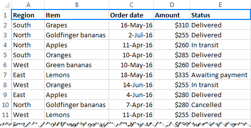
Once the column headings are in pace, select any cell within your dataset, and use one of the following methods to insert filter.
3 ways to add filter in Excel
- On the Data tab, in the Sort & Filter group, click the Filter button.

- On the Home tab, in the Editing group, click Sort & Filter > Filter.

- Use the Excel Filter shortcut to turn the filters on/off: Ctrl+Shift+L
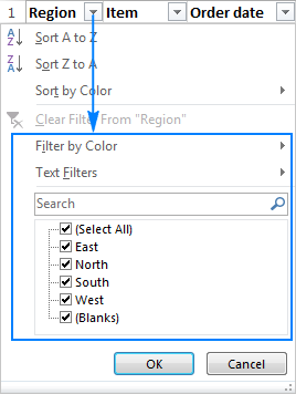
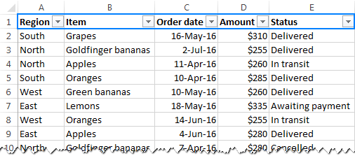
Whatever method you use, the drop-down arrows will appear in each of the header cells:
How to apply filter in Excel
A drop-down arrow ![]() in the column heading means that filtering is added, but not applied yet. When you hover over the arrow, a screen tip displays (Showing All).
in the column heading means that filtering is added, but not applied yet. When you hover over the arrow, a screen tip displays (Showing All).
To filter data in Excel, do the following:
- Click the drop-down arrow for the column you want to filter.
- Uncheck the Select All box to quickly deselect all data.
- Check the boxes next to the data you want to display, and click OK.
For example, this is how we can filter data in the Region column to view sales only for East and North:
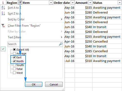
Done! The filter is applied to column A, temporarily hiding any regions other than East and North.
The drop-down arrow in the filtered column changes to the Filter button ![]() , and hovering over that button displays a screen tip indicating which filters are applied:
, and hovering over that button displays a screen tip indicating which filters are applied:

Tip. To quickly find the number of filtered / visible rows, just take a look at the Excel status bar.
Filter multiple columns
To apply Excel filter to multiple columns, just repeat the above steps for as many columns as you want.
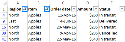
For example, we can narrow down our results to only show Apples for the East and North regions. When you apply multiple filters in Excel, the filter button appears in each of the filtered columns:
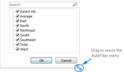
Tip. To make the Excel Filter window wider and/or longer, hover over the grip handle at the bottom, and as soon as the double-headed arrow appears, drag it down or to the right.
Filter blank / non-blank cells
To filter data in Excel skipping blanks or non-blanks, do one of the following:
To filter out blanks, i.e. display non-blank cell, click the auto-filter arrow, make sure the (Select All) box is checked, and then clear (Blanks) at the bottom of the list. This will display only those rows that have any value in a given column.
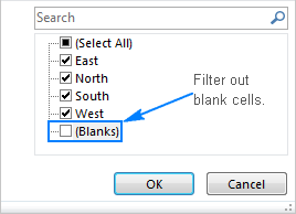
To filter out non-blanks, i.e. display only empty cells, clear (Select All), and then select (Blanks). This will display only the rows with an empty cell in a given column.
Notes:
- The (Blanks) option is available only for columns that contain at least one empty cell.
- If you want to delete blank rows based on some key column, you can filter out non-blanks in that column, select the filtered rows, right-click the selection, and click Delete row. If you want to delete only those rows that are completely blank and leave the rows with some content and some empty cells, check out this solution.
How to use filter in Excel
Apart from basic filtering options discussed above, AutoFilter in Excel provides a number of advanced tools that can help you filter specific data types such as text, numbers and dates exactly the way you want.
Notes:
- Different Excel filter types are mutually exclusive. For example, you can filter a given column by value or by cell color, but not by both at a time.
- For correct results, do not mix different value types in a single column because only one filter type is available for each column. If a column contains several types of values, the filter will be added for the data that occurs the most. For example, if you store numbers in a certain column but most of the numbers are formatted as text, Text Filters will appear for that column but not Number Filters.
And now, let's have a closer look at each option and see how you can create a filter most suited for your data type.
Filter text data
When you want to filter a text column for something very specific, you can leverage a number of advanced options provided by Excel Text Filters such as:
- Filter cells that begin with or end with a specific character(s).
- Filter cells that contain or do not contain a given character or word anywhere in the text.
- Filter cells that are exactly equal or not equal to a specified character(s).
As soon as you add a filter to a column containing text values, Text Filters will appear automatically in the AutoFilter menu:
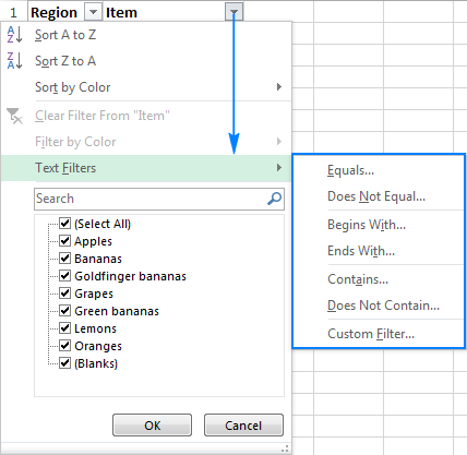
For instance, to filter out rows containing Bananas, do the following:
- Click the drop-down arrow in the column heading, and point to Text Filters.
- In the drop-down menu, select the desired filter (Does Not Contain… in this example).
- The Custom AutoFilter dialog box will show up. In the box to the right of the filter, type the text or select the desired item from the dropdown list.
- Click OK.
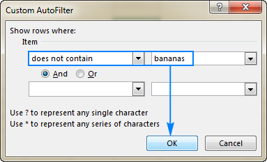
As the result, all of the Bananas rows, including Green bananas and Goldfinger bananas, will be hidden.
Filter column with 2 criteria
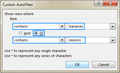
To filter data in Excel with two text criteria, perform the above steps to configure the first criteria, and then do the following:
- Check And or Or radio button depending on whether both or either criterion should be true.
- Select the comparison operator for the second criterion, and enter a text value in the box right to it.
For example, this is how you can filter rows that contain either Bananas or Lemons:
How to create filter in Excel with wildcard characters
If you don't remember exact search or want to filter rows with similar information, you can create a filter with one the following wildcard characters:
| Wildcard character | Description | Example |
| ? (question mark) | Matches any single character | Gr?y finds "grey" and "gray" |
| * (asterisk) | Matches any sequence of characters | Mid* finds "Mideast" and "Midwest" |
| ~ (tilde) followed by *, ?, or ~ | Allows filtering cells that contain a real question mark, asterisk, or tilde. | What~? finds "what?" |
Tip. In many cases, you can use the Contains operator instead of wildcards. For example, to filter cells containing all sorts of Bananas, you can either select the Equals operator and type *bananas*, or use the Contains operator and simply type bananas.
How to filter numbers in Excel
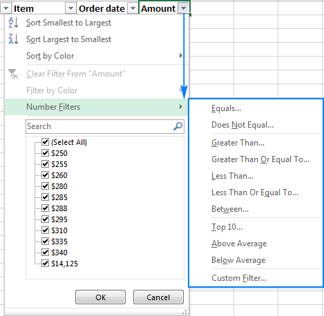
Excel's Number Filters allow you to manipulate numeric data in a variety of ways, including:
- Filter numbers equal or not equal to a certain number.
- Filter numbers, greater than, less than or between the specified numbers.
- Filter top 10 or bottom 10 numbers.
- Filter cells with numbers that are above average or below average.
The following screenshot shows the whole list of number filters available in Excel.
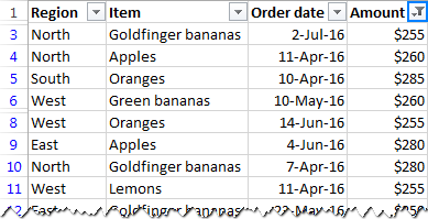
For example, to create a filter that displays only orders between $250 and $300, proceed with these steps:
- Click the autofilter arrow in the column header, and point to Number Filters.
- Choose an appropriate comparison operator from the list, Between… in this example.
- In the Custom AutoFilter dialog box, enter the lower bound and upper bound values. By default, Excel suggests using "Greater than or equal to" and "Less than or equal to" comparison operators. You can change them to "Greater than" and "Less than' if you don't want the threshold values to be included.
- Click OK.

As the result, only orders between $250 and $300 are visible:
How to filter dates in Excel
Excel Date Filters provide the greatest variety of choices that let you filter records for a certain time period quickly and easily.
By default, Excel AutoFilter groups all dates in a given column by a hierarchy of years, months, and days. You can expand or collapse different levels by clicking the plus or minus signs next to a given group. Selecting or clearing a higher level group selects or clears data in all nested levels. For instance, if you clear the box next to 2016, all dates within the year 2016 will be hidden.
In addition, Date Filters allow you to display or hide data for a particular day, week, month, quarter, year, before or after a specified date, or between two dates. The screenshot below demonstrates all available date filters:
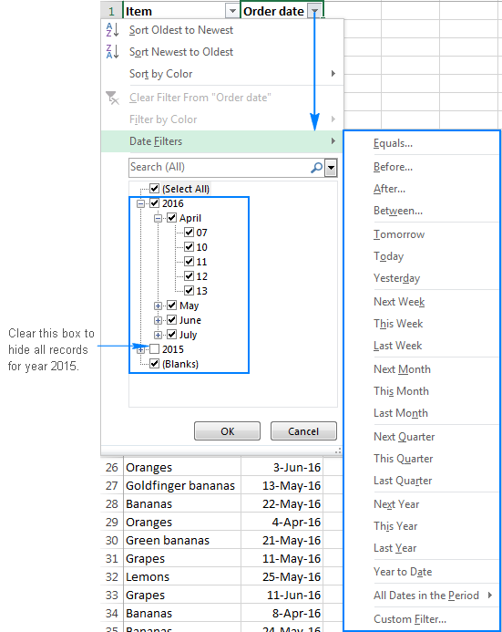
In most cases, Excel filter by date works in a single click. For instance, to filter rows containing records for the current week, you simply point to Date Filters and click This Week.
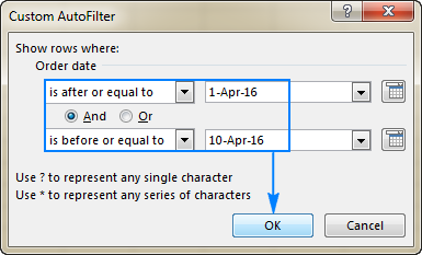
If you select the Equals, Before, After, Between operator or Custom Filter, the already familiar Custom AutoFilter dialog window will show up, where you specify the desired criteria.
For example, to display all items for the first 10 days of April 2016, click Between… and configure the filter in this way:
How to filter by color in Excel
If the data in your worksheet is formatted manually or through conditional formatting, you can also filter that data by color.
Clicking the autofilter drop-down arrow will display Filter by Color with one or more options, depending on which formatting is applied to a column:
- Filter by cell color
- Filter by font color
- Filter by cell icon
For example, if you formatted cells in a given column with 3 different background colors (green, red and orange) and you want to display only orange cells, you can get it done in this way:
- Click the filter arrow in the header cell, and point to Filter by Color.
- Click the desired color - orange in this example.
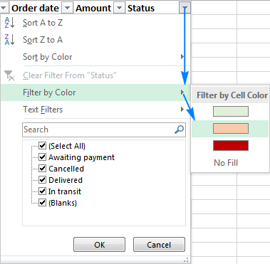
Voila! Only values formatted with the orange font color are visible and all other rows are temporarily hidden:
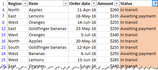
For more information, please see How to filter and sort by cell color in Excel.
How to filter in Excel with search
Beginning with Excel 2010, the Filter interface includes a search box that facilitates navigation in large data sets enabling you to swiftly filter rows containing an exact text, number, or date.
Suppose you want to view the records for all "east" regions. Just click the autofilter dropdown, and start typing the word "east" in the search box. Excel Filter will immediately show you all items that match the search. To display only those rows, either click OK in the Excel AutoFilter menu, or press the Enter key on your keyboard.
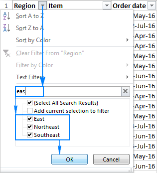
To filter multiple searches, apply a filter according to your first search term as demonstrated above, then type the second term, and as soon as the search results appear, select the Add current selection to filter box, and click OK. In this example, we are adding "west" records to the already filtered "east" items:
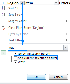
That was pretty fast, wasn't it? Only three mouse clicks!
Filter by selected cell value or format
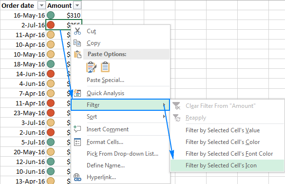
One more way to filter data in Excel is to create a filter with the criteria equal to the contents or formats of the selected cell. Here's how:
- Right click a cell containing the value, color, or icon you want to filter your data by.
- In the context menu, point to Filter.
- Select the desired option: filter by selected cell's value, color, font color, or icon.
In this example, we are filtering data by the selected cell's icon:
Re-apply a filter after changing data
When you edit or delete data in filtered cells, Excel AutoFilter does not update automatically to reflect the changes. To re-apply the filter, click any cell within your dataset, and then either:
- Click Reapply on the Data tab, in the Sort & Filter group.

- Click Sort & Filter > Reapply on the Home tab, in the Editing group.

How to copy filtered data in Excel
The fastest way to copy a filtered data range to another worksheet or workbook is by using the following 3 shortcuts.
- Select any filtered cell, and then press Ctrl + A to select all filtered data including column headers.
To select filtered data excluding column headers, select the first (upper-left) cell with data, and press Ctrl + Shift + End to extend the selection to the last cell.
- Press Ctrl + C to copy the selected data.
- Switch to another sheet/workbook, select the upper-left cell of the destination range, and press Ctrl+V to paste the filtered data.
Note. Usually, when you copy the filtered data elsewhere, filtered-out rows are omitted. In some rare cases, mostly on very large workbooks, Excel may copy hidden rows in addition to visible rows. To prevent this from happening, select a range of filtered cells, and press Alt + ; to select only visible cells ignoring hidden rows. If you're not accustomed to using keyboard shortcuts, you can utilize the Go To Special feature instead (Home tab > Editing group > Find & Select > Go to Special... > Visible Cells only).
How to clear filter
After applying a filter to a certain column, you may want to clear it to make all information visible again or filter your data in a different way.
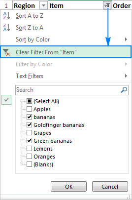
To clear a filter in a certain column, click the filter button in the column's header, and then click Clear Filter from <Column name>:
How to remove filter in Excel
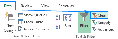
To remove all filters in a worksheet, do one of the following:
- Go to the Data tab > Sort & Filter group, and click Clear.
- Go to the Home tab > Editing group, and click Sort & Filter > Clear.
Filter not working in Excel
If Excel's AutoFilter stopped working partway down a worksheet, most likely it's because some new data has been entered outside the range of filtered cells. To fix this, simply re-apply filter. If that does not help and your Excel filters are still not working, clear all filters in a spreadsheet, and then apply them anew. If your dataset contains any blank rows, manually select the entire range using the mouse, and then apply autofilter. As soon as you do this, the new data will be added to the range of filtered cells.
Basically, this is how you add, apply and use filter in Excel. But there is much more to it! In the next tutorial, we will explore and capabilities of Advanced Filter and see how to filter data with multiple sets of criteria. Please stay tuned!
 by
by
16 comments
I applied A to Z filter in my Workbook and after that i saved it and my coordinated data has been unpositioned now. So please tell me the option by applying that i can get my original data as same postion back.
Hi,
If you used the recommendations from this article, then pay attention to the paragraph — How to clear filter
HI, My question is, How to remove advanced filter data in a particular cell
Hello!
Please note that the advanced filter is applied to the data table, not to a particular cell. For me to give you a more precise answer, please describe your problem in more detail.
Is there a way to add a filter to a specific area? e.g A1 - C50 and then it would only filter that area.
Antony, highlight the area you want to filter before you press the filter button.
Hi,
Thank you for sharing.
Do you know how to find which column is filtered? For example there are many columns (A1:A300)and some of them is filtered. How to find the filtered one?
Thank u in advance..
The second argument identifies the column to be filtered by. If I use the following function:
=filter(A:AX,D:D=5)
The funtions is saying that it is searching all rows down columns from A to AX, and looking for 5 as the value in column D.
Likely A1:A300 is the data range being filtered, the second argument should identify the column where values are looked for.
Please advise if I can have some button/slicer that can enable me to switch between two different filters for pivot table.
I have prepared a sales analysis pivot chart. I want an option to switch between total quantity or total sales figure on pivot chart.
How do I do it?
Hi Osama, write "total quantity" in a cell and write "total sales" in another cell (beside the first one cell or below or wherever you want). Right click the cell you wrote "total quantity" in - select "Hyperlink" - under "Link to:" clink on "Place in This Document" - write the cell name of the "total quantity column or pivot table if both are in different pivots" in "Type the cell reference" e.g. D25 - click OK and the shortcut for "total quantity" is created, now do the same for "total sales"
What is the shortcut for "Text Filter column with 2 criteria"
I would like to go to "Contains and Contains" option by one click but I was not able to find it. Can you please explain me how to create shortcut for that? Even this can be with macros.
Use the text filter option and choose contains from the popup
A new window Custom Autofilter is there wherein you enter both the "contains" with conditions of "And" and click OK.
This should work for sure.
please advise me
if too many names - data is available in one sheet.
and if we need to add some data under anyone's name.
should i filter according to names and update the data under that.
when i do that,
after selecting all data
the new added data comes at the end of the excel sheet.
please advise
Hi Sameer, make a column for numbering (unique numbers) and give numbers 1, 2, 3, 4... etc. for names and give 1.1, 1.2, 2.1, 2.2, 2.3... etc. for other related data of each name and in last of your data entry sort as the Smallest to Biggest and you will get each related data for a single person under his name.
e.g. let suppose A and B are the names and AA & BB are the father names that we need to put under the name of their sons. A is son of AA and B is son of BB. The unique number for A will be 1, for AA will be 1.1 and for B will be 2, for BB will be 2.2. And let suppose after the father name you need to add their age, the number for age of A will be 1.3 and for B will be 2.3.
I hope it helps you with what you are seeking.
Hi Dear,
Is there a formula for below task?
Suppose our organization works in 3 (A, B and C) Schools. And for schools, our organization only gives School Seminars and Refresher School Seminars about Disaster Risk Reduction.
e.g. First Seminars are conducted in all schools but Refresher Seminar is just conducted for School B in a specific date.
I need a formula for Gap Analysis using the dates of the seminars, that will only take the last dates. Means "If the cell "Refresher Seminar Date" is empty, the formula will take the date from the cell "First Seminar Date" but if the cell "Refresher Seminar Date" has data, the cell won't take the date from " First Seminar" but it will automatically take the Date from the cell "Refresher Seminar Date".
Many thanks for your nice work, please keep it up! :)
Dear Suliman,
Supposing "First Seminar Date" is in column A, and "Refresher Seminar Date" is in column B, you can use the following formula:
=IF(B2<>"", B2, A2)