The tutorial shows how to use the LEFT function in Excel to get a substring from the beginning of the text string, extract text before a certain character, force a Left formula to return a number, and more.
Among many different functions that Microsoft Excel provides for manipulating text data, LEFT is one of the most widely used. As its name suggests, the function allows you to extract a certain number of characters starting at the left side of a text string. However, Excel LEFT is capable of much more than its pure essence. In this tutorial, you will find a couple of basic Left formulas to understand the syntax, and then I will show you a few ways in which you can take the Excel LEFT function well beyond its basic usage.
Excel LEFT function - syntax
The LEFT function in Excel returns the specified number of characters (substring) from the start of a string.
The syntax of the LEFT function is as follows:
Where:
- Text (required) is the text string from which you want to extract a substring. Usually it is supplied as a reference to the cell containing the text.
- Num_chars (optional) - the number of characters to extract, starting on the left side of the string.
- If num_chars is omitted, it defaults to 1, meaning that a Left formula will return 1 character.
- If num_chars is greater than the total length of text, a Left formula will return all of text.
For example, to extract the first 3 characters from the text in cell A2, use this formula:
=LEFT(A2, 3)
The following screenshot shows the result:

Important note! LEFT belongs to the category of Text functions, therefore the result of a Left formula is always a text string, even if the original value from which you extract characters is a number. If you are working with a numeric dataset and want the LEFT function to return a number, use it in conjunction with the VALUE function as demonstrated in this example.
How to use LEFT function in Excel - formula examples
Apart from extracting text from the left of a string, what else can the LEFT function do? The following examples show how you can use LEFT in combination with other Excel functions to solve more complex tasks.
How to extract a substring before a certain character
In some cases, you may need to extract the part of the text string that precedes a specific character. For example, you may want to pull the first names from a column of full names or get the country codes from a column of phone numbers. The problem is that each name and each code contains a different number of characters, and therefore you cannot simply supply a predefined number to the num_chars argument of your Left formula like we did in the above example.
If the first and last names are separated by a space, the problem boils down to working out the position of the space character in a string, which can be easily done by using either SEARCH or FIND function.
Supposing the full name is in cell A2, the position of the space is returned by this simple formula: SEARCH(" ",A2)). And now, you embed this formula in the num_chars argument of the LEFT function:
=LEFT(A2, SEARCH(" ", A2))
To improve the formula a bit further, get rid of the trailing space by subtracting 1 from the Search formula result (not visible in cells, trailing spaces may cause many problems especially if you plan to use the extracted names in other formulas):
=LEFT(A2, SEARCH(" ", A2)-1)
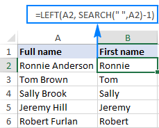
In the same fashion, you can extract the country codes from a column of telephone numbers. The only difference is that you use the Search function to find out the position of the first hyphen ("-") rather than a space:
=LEFT(A2, SEARCH("-", A2)-1)
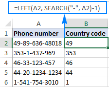
Wrapping up, you can use this generic formula to get a substring that precedes any other character:
How to remove the last N characters from a string
You already know how to use the Excel LEFT function to get a substring from the start of a text string. But sometimes you may want to do something different - remove a certain number of characters from the end of the string and pull the rest of the string into another cell. For this, use the LEFT function in combination with LEN, like this:
The formula works with this logic: the LEN function gets the total number of characters in a string, then you subtract the number of unwanted characters from the total length, and have the LEFT function return the remaining characters.
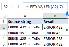
For example, to remove the last 7 characters from text in A2, use this formula:
=LEFT(A2, LEN(A2)-7)
As shown in the screenshot below, the formula successfully cuts off the " - ToDo" postfix (4 letters, a hyphen and 2 spaces) from the text strings in column A.
How to force the LEFT function to return a number
As you already know, the Excel LEFT function always returns text, even when you are pulling a few first digits from a number. What it means to you is that you won't be able to use the results of your Left formulas in calculations or in other Excel functions that operate on numbers.
So, how do you make Excel LEFT to output a number rather than a text string? Simply by wrapping it in the VALUE function, which is designed to convert a string representing a number to a number, like this: VALUE(LEFT())
For example, to extract the first 2 characters from the string in A2 and convert the output into numbers, use this formula:
=VALUE(LEFT(A2,2))
The result will look something similar to this:
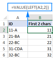
As you can see in the screenshot above, the numbers in column B obtained with a Value Left formula are right-alighted in cells, as opposed to left-aligned text in column A. Since Excel recognizes the output as numbers, you are free to sum and average those values, find the min and max value, and perform any other calculations.
These are just a few of many possible uses of LEFT in Excel. To have a closer look at the formulas discussed in this tutorial, you are welcome to download the Excel LEFT function sample worksheet.
For more Left formula examples, please check out the following resources:
Excel LEFT function not working - reasons and solutions
If the Excel LEFT function does not work properly in your worksheets, it's most likely because of one of the following reasons.
1. Num_chars argument is less than zero
If your Excel Left formula returns the #VALUE! error, the first thing for you to check is the value in the num_chars argument. If it's a negative number, just remove the minus sign and the error will be gone (of course, it's very unlikely that someone will put a negative number there of purpose, but to err is human :)
Most often, the VALUE error occurs when the num_chars argument is represented by another function. In this case, copy that function to another cell or select it in the formula bar and press F9 to see what it equates to. If the value is less than 0, then check the function for errors.
To better illustrate the point, let's take the Left formula we've used in the first example to extract the country phone codes: LEFT(A2, SEARCH("-", A2)-1). As you may remember, the Search function in the num_chars argument calculates the position of the first hyphen in the original string, from which we subtract 1 to remove the hyphen from the final result. If I accidentally replace -1, say, with -11, the formula would through the #VALUE error because the num_chars argument equates to a negative numbers:

2. Leading spaces in the original text
In case your Excel Left formula fails for no obvious reason, check the original values for leading spaces. If you have copied your data from the web or exported from another external source, many such spaces may lurk unnoticed before the text entries, and you will never know they are there until something goes wrong. The following image illustrates the problem:
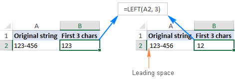
To get rid of the leading spaces in your worksheets, use the Excel TRIM function or the Trim spaces tool.
3. Excel LEFT does not work with dates
If you attempt use the Excel LEFT function to get an individual part of a date (such as day, month or year), in most cases you will only retrieve the first few digits of the number that represents that date. The point is that in Microsoft Excel, all dates are stored as integers representing the number of days since January 1, 1900, which is stored as number 1 (for more information, please see Excel date format). What you see in a cell is just a visual representation of the date and its display can easily be changed by applying a different date format.
For example, if you have the date 11-Jan-2017 in cell A1 and you try to extract the day by using the formula LEFT(A1,2), the result would be 42, which is the first 2 digits of number 42746 that represents January 11, 2017 in the internal Excel system.
To extract a specific part of a date, use one of the following functions: DAY, MONTH or YEAR.
In case your dates are entered as text strings, the LEFT function will work without a hitch, as shown in the right part of the screenshot:
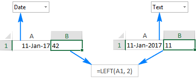
This is how you use the LEFT function in Excel. I thank you for reading and hope to see you again next week.
 by
by
95 comments
I need help with a formula that used to work in older versions of Excel.
=IF(LEFT(A3, 6)=L2,K3,0)
the IF(left(A3, 6) is stating true but when I add = to L2 it becomes false even though the value is the same in the A3 and L2 field.
Hello Nicole!
It's possible one of the cells contains non-printable characters. I recommend trying these instructions: How to remove special (unwanted) characters from string in Excel.
Need help with a formula. lets say the cells starts with 1C,2C,3C and so on. so i used to use " =--LEFT(A6,FIND("C",A6)-1) " formula to seperate the numbers infront of "C" . Now i have 1D,2D,3D along with the 1C,2C,3C beginings... what do i do to fix this formula?
Hi! To remove last character from text and convert it to a number, try this formula:
=--LEFT(A6,LEN(A6)-1)
LEFT function determines the number of characters in a text string.
Can someone help me on to extract the text from right to left with the space between the number and text?
example: XYZ-OP-7284-L-052-22 XYZ CN.2020-S006 Expanded Combined Schedule Rev. A Summary
Result must be: Expanded Combined Schedule Rev. A Summary
another example: XYZ-OP-7284-L-149-22 Change Notice - Additional Requirement for Construction of Perimeter Drain
Result must be: Change Notice - Additional Requirement for Construction of Perimeter Drain
Hello Arnold!
If I understand your question correctly, you want to extract text after last digit in text. To find the position of last digit in text, you can try this formula:
=MAX(IF(ISNUMBER(--MID(A1, ROW(INDIRECT("1:"&LEN(A1))), 1)), ROW(INDIRECT("1:"&LEN(A1))), 0))
MID(A1, ROW(INDIRECT(“1:”&LEN(A1))), 1) - retrieves each character from the string in cell A1.
ISNUMBER(--MID(...)) - checks if this character is a digit. Read more: Excel ISNUMBER function with formula examples.
ROW(INDIRECT(“1:”&LEN(A1)))) - creates an array of character positions. For more information: Excel INDIRECT function - basic uses and formula examples.
MAX(...) - finds the maximum value among digit positions, i.e. last digit.
You can then use MID function to extract all characters starting from this position.
=MID(A1,MAX(IF(ISNUMBER(--MID(A1, ROW(INDIRECT("1:"&LEN(A1))), 1)), ROW(INDIRECT("1:"&LEN(A1))), 0))+1,300)
Hello!
How do I pull everything to the left of the first number in a string of text? I have the =RIGHT formula and now need everything to the left to separate out into 2 columns. My right formula is =RIGHT(A2, LEN(A2) - MIN(FIND({0,1,2,3,4,5,6,7,8,9}, A2&"0123456789")) + 1) and it works.
Thanks in advance!
Hello Danielle!
To extract all characters to the left of the first digit, use LEFT function instead RIGHT
=LEFT(A2, LEN(A2) - MIN(FIND({0,1,2,3,4,5,6,7,8,9}, A2&"0123456789")))
Hi, happy holidays! I have a list of criteria where one column contains either a letter number combination or just numbers and I need a formula that recognizes if the first 2 characters are letters. The only way I've been able to do it so far is "LEFT(Table1!J2;2)="AA"; LEFT(Table1!J2;2)="XY")" etc.. The letters are never the same but always at the front and there are very many. Is there a way to have Excel recognize I'm looking for the first 2 characters that are not numbers?
Hello Sissi!
Extract the first two characters from the text using the MID function. Determine whether these characters are numbers using the ISNUMBER function. If both of these characters are not numbers, the SUMPRODUCT function will return the number 1, and the IF function will return the text “Not numbers”. The formula might look like this:
=IF(SUMPRODUCT(--ISNUMBER(MID(A1,{1,2},1))),"Not numbers","")
=LEFT(B482,2)&MID(B4822,5)
formula not working
how to write a right method
Hi! Read carefully here how to correctly use the MID function: Excel MID function – extract text from the middle of a string.
Hello,
I am using the the =LEFT (C2, SEARCH(" ", C2)-1) to create a new column.
The data extracted into the new column is a date MM/DD/YYYY
I now need to take that date is C2 and subtract it from another date in a different column. When using the simple format of for example =E2-C2 it is giving me a #VALUE! error. I made sure my date format is all matching as well as looked into the 'evaluate formula' but still can't seem to fix the issue.
Hello! The date you extracted with the LEFT function is written as text. The LEFT function always returns text. Convert this text to a date using any of the methods described in this manual: How to convert text to date in Excel. For example,
=DATEVALUE(LEFT(C2,SEARCH(" ",C2)-1))
You will then be able to calculate the date difference.
Need to sum a vertical range whose criteria of the other column starts with the letter B, for example...
left for a range works or not
Hi! To sum values based on partial match, follow these instructions: SUMIF formulas with wildcard characters.
I am trying to separate a percent number from a course in a cell, when there are multiple terms.
For example Cells may be
88%- ENGL100, 100%- MATH111
92%- BUSN115, 75%- ENGL100
72%- ENGL100
I only was to see the percent for one class, so I can then create an if statement to find the letter grade.
How can I return only the 4 characters, or numbers before ENGL100- if the order of the classes may differ from cell to cell?
Hi! You can get all characters before "-" using the LEFT and SEARCH functions.
=LEFT(A1,SEARCH("-",A1)-1)
Read this article for more information: Excel FIND and SEARCH functions with formula examples.
Hi, can you please help me with a formula for the below
EX : i have column A with values like CAIU1234567, SEGU1234567, TTNU1234567, CRXU1234567, CAIU8910111
column B with values like Cargo, Container, Box
I need result in column C as Cargo for CAIU and Box for SEGU & TTNU and Container for CRXU
You can use the SEARCH function to find partial text matches.
For example:
=IF(ISNUMBER(SEARCH("CAIU",A1)),"Cargo",IF(ISNUMBER(SEARCH("SEGU",A1)),"Box"),"")
For more information, please read: How to find substring in Excel
Hi,
If I have a name & surname, and I just want the most left letter of the combined. For example some has 2 words, like Pete Sampras, then it would make "PS". But some have more, like Pete Steff Sampras. Now it would be "PSS". Some has more than 2 or 3 words, so how would I go about it?
How will this function of formula looks like
Hello!
You can extract all pattern matches from text with the custom function RegExpExtract. Use the examples and instructions in this guide: Regex to extract strings in Excel (one or all matches).
Formula example:
=CONCAT(RegExpExtract(A1,"[A-Z] *"))
You can get more options to extract text by pattern by using Regex Tools. It is available as a part of our Ultimate Suite for Excel that you can install in a trial mode and check how it works for free.
Cell A1(Employee First Name): JOHN
Cell A2(Employee Last Name): DEY
Cell A3(DOB, month and date): 1027 (27th Oct)
Cell A4 should be a combination of 14 characters which will be "MMDDFFFFFLLLLL"
-MM - Month
-DD - Date
-FFFFF and LLLLL: First five letters of the first and last name, if its short by five characters then last characters should be filled with letter X to make it 5 length character
Here, the Output should be 1027JOHNXDEYXX
Hello!
If I understand your task correctly, the following formula should work for you:
=A3&LEFT(A1,5) & LEFT(A2,5) & REPT("X",MAX(0,5-LEN(A2)))
Hi Alex, this is working for me ! Appreciate your help ! Thank you so much !
I have just added "& REPT("X",MAX(0,5-LEN(A1)))" this part to complete the formula
=A3&LEFT(A1,5) & REPT("X",MAX(0,5-LEN(A1))) & LEFT(A2,5) & REPT("X",MAX(0,5-LEN(A2)))
Hi Alex,
Kindly assist with the excel formula to get the mentioned output.
Regards, Vasim
Is there a formula that can extract the next four digits after finding/reading '8420' in a cells text string.
Hello!
Extract all numbers from the text as described in this instruction: How to get number from any position in a string.
Find the digit position "8420" using the SAERCH function. Then use the MID function to get 4 digits after this position.
=MID(SUMPRODUCT(MID(0&A2, LARGE(INDEX(ISNUMBER(--MID(A2, ROW(INDIRECT("1:"&LEN(A2))), 1)) * ROW(INDIRECT("1:"&LEN(A2))), 0), ROW(INDIRECT("1:"&LEN(A2))))+1, 1) * 10^ROW(INDIRECT("1:"&LEN(A2)))/10),SEARCH("8420",SUMPRODUCT(MID(0&A2, LARGE(INDEX(ISNUMBER(--MID(A2, ROW(INDIRECT("1:"&LEN(A2))), 1)) * ROW(INDIRECT("1:"&LEN(A2))), 0), ROW(INDIRECT("1:"&LEN(A2))))+1, 1) * 10^ROW(INDIRECT("1:"&LEN(A2)))/10))+4,4)
Thanks for the very quick response...
Unfortunately, the formula doesn't seem to cope with the following example returning a #VALUE! error - please advise if possible.
Cell data:
Axxx Cxxx 02/10/22 - 1008001129815 - 842019000 recode from 900000.5000002 to 900001.50000001
Please also note I require the 8420 to be included in the returned value (which should be the next 5 digits not 4 as previously requested ...
As such I have tweaked the formula provided as follows, which works for 95% of the dataset being analysed
="8420"&(MID(SUMPRODUCT(MID(0&A2, LARGE(INDEX(ISNUMBER(--MID(A2, ROW(INDIRECT("1:"&LEN(A2))), 1)) * ROW(INDIRECT("1:"&LEN(A2))), 0), ROW(INDIRECT("1:"&LEN(A2))))+1, 1) * 10^ROW(INDIRECT("1:"&LEN(A2)))/10),SEARCH("8420",SUMPRODUCT(MID(0&A2, LARGE(INDEX(ISNUMBER(--MID(A2, ROW(INDIRECT("1:"&LEN(A2))), 1)) * ROW(INDIRECT("1:"&LEN(A2))), 0), ROW(INDIRECT("1:"&LEN(A2))))+1, 1) * 10^ROW(INDIRECT("1:"&LEN(A2)))/10))+4,5))
Hi!
You didn't provide details on how you want to extract the numbers. For your example, use the simple MID formula
=MID(A2,SEARCH("8420",A2),9)
What formula will be used in Excel to get the value left in the column B2 to E2 other than the value which is taken in the column by column A2?
For Exam:
A2 = Finish Powerball All In 1 Max 60 Dishwasher Tablets Value Pack
B2 = Finish
C2 = Powerball
D2 = 60 Dishwasher
E2 = Tablets
G2 = ???? (rest of title value)
(All In 1 Max, Value Pack)
how to find by formula in excle
Hi!
To remove a few words from text, use the nested SUBSTITUTE function:
=SUBSTITUTE(SUBSTITUTE(SUBSTITUTE(SUBSTITUTE(A2,B2,""),C2,""),D2,""),E2,"")
This should solve your task.
Thanks a lot :)
I want to delete some letters in the right position. like the following example:
LITE TESSIAN 10P S
LITE TESSIAN 50P S +
LITE TESSIAN 40P S+
i want to remove the letters "S" , "S+" and "S +".
please help. thank you
You can use LEFT Function with Len.
For Example:
Products Formula
BB SEAMUSS 100X S+ =LEFT(A2,LEN(A2)-3)
BB SEAMUSS 140X S +
LITE TESSIAN 10P S
LITE TESSIAN 50P S +
LITE TESSIAN 40P S+
Please check and Comments
Hello!
If you want to remove specific characters from text, use this guide: Replace character(s) with nothing.
If this is not what you wanted, please describe the problem in more detail.
BB SEAMUSS 100X S+
BB SEAMUSS 140X S +
LITE TESSIAN 10P S
LITE TESSIAN 50P S +
LITE TESSIAN 40P S+
i want to remove the letters "S" , "S+" and "S +".
please help. thank you
I've been fighting with EXACT, LEFT and data validation. I want to ensure that my spreadsheet users only enter a postcode into a particular cell. The postcodes can begin with BR, BA or GL and would be 6 or 7 characters long in total. Is there a way to enter that as a formulae into Data Validation using EXACT/LEFT ? Thanks in advance
Hello!
Use the data validation tool with this formula:
=SUM(--(LEFT(A1,2)={"BR","BA","GL"}))*(LEN(A1)>5)*LEN(A1)<8
I hope my advice will help you solve your task.
Hi Alexander,
Thanks for your help with this, but I am unable to apply this formulae within custom Data Validation. I get this message.
"You may not use reference operators (such as unions, intersections, and ranges), array constants, or the LAMBDA function for Data Validation criteria"
Hi!
Replace the array of values with the sum of conditions by logic OR
=((LEFT(A1,2)="BR")+(LEFT(A1,2)="BA")+(LEFT(A1,2)="GL"))*(LEN(A1)>5)*(LEN(A1)<8)
This should solve your task.
Alexander - you are a STAR! Works a treat. Thank you! Now I just need to apply a slight tweak as if a user enters BS10 3FG , or GL1 3DD for example, it will return an error. If they enter BS103FG or GL13DD it accepts it. This is right, based on what you have created for me.
Would you use the SUBSTITUTE formulae to remove any space entered and would this have to go at the beginning of the formulae so the other validation happens after?
I am going to state "no spaces" on the Form next to the cell itself but know users will still put them!
Thanks again :)
Hello!
Add a space check to your formula using the SEARCH function.
=SUM(--(LEFT(A1,2)={"BR","BA","GL"}))*(LEN(A1)>5)*(LEN(A1)<8)*ISERROR(SEARCH(" ",A1))
This should solve your task.
Yet again - exactly what I asked for - THANKS ! At the risk of pushing my luck......
I realise that the system that will read the completed form insists that postcodes with 6 digits are input with a space, and those with 7 digits do not have a space. Again, I can state this on the form but wonder if there is an extra bit I can add to the code that would take this into account, and make the user enter a space if 6, and not if 7 . Aware this is starting to become very drawn out formulae, but cannot think of a way round it that doesn't rely on users following instructions!
Hello!
You can automatically change the value in a cell using a VBA macro. Or use input massage in Data Validation to warn the user to enter 7 digits.
Boy do I love this website. Can I ask how to write a formula that would count uppercase characters before the first space? I tried the following but didn't work quite right:
=LEN(LEFT(SUMPRODUCT(LEN(A1)-LEN(SUBSTITUTE(A1,CHAR(ROW(INDIRECT("65:90"))),""))))-SEARCH(" ",A1))
Hello!
Please try the following formula:
=SUM(--(NOT(ISNUMBER(--MID(LEFT(A1,SEARCH(" ",A1,1)), ROW(INDIRECT("$1:$"&(SEARCH(" ",A1,1)-1))),1)))*(EXACT(MID(LEFT(A1,SEARCH(" ",A1,1)), ROW(INDIRECT("$1:$"&(SEARCH(" ",A1,1)-1))),1), UPPER(MID(LEFT(A1,SEARCH(" ",A1,1)), ROW(INDIRECT("$1:$"&(SEARCH(" ",A1,1)-1))),1))))))
Can I use LEFT as part of a calculation. IF the first 2 letters in column $A20 are ii, C20= B20+C19, otherwise C20=C19.
Hi!
The article describes in detail how to use the LEFT function. Use LEFT function together with IF function.
=IF(LEFT(A20,2)="ii",B20+C19,C19)
I have a column with 2 or 3 text characters followed by numbers and want to extract the text only. Typically there will be 3 text characters, but occasionally only 2 text characters. I want to extract only the text from the string. so if I have MM10103, I want to get the value MM, but if I have XYZ10103 I want the value XYZ extracted. I have used LEFT(A1,3) and get MM1 in the first case, and XYZ in the second. How do I modify this to deliver correct 2 or 3 digit string of text only values?
Value Prefix
AC10103 AC
CCA0101 CCA
CCM0501 CCM
CYM0101 CYM
CYQ0010 CYQ
Thanks
Hello!
You can extract only letters without numbers using this formula:
=SUBSTITUTE((CONCAT(IF(NOT(ISNUMBER(--MID(A3,ROW($1:$94),1))),MID(A3,ROW($1:$94),1),"")))," ","")
You can also use regular expressions. See the article for instructions and examples: Regex to extract strings in Excel (one or all matches).
Hello, i'm trying to create a formula for these two columns to then be four... I can't seem to use the left/right formula as not all columns have a "," character. I know you can use text to column but want something automated
A Bucket_1 [100/-100]
Bucket_1 [100/-100]
Bucket_1,Bucket_2 [100/-100],[200/-200]
Bucket_2,Bucket_3 [200/-200],[400/-400]
Bucket_3 [400/-400]
B Bucket_1 [100/-100]
Bucket_1 [100/-100]
Bucket_1 Bucket_2 [100/-100] [200/-200]
Bucket_2 Bucket_3 [200/-200] [400/-400]
Bucket_3 [400/-400]
Hello!
You use space and comma as a separator. I don’t think you can divide your data into 4 columns using a formula. I recommend the Split Text tool, which can do this in a couple of clicks. It is available as a part of our Ultimate Suite for Excel that you can install in a trial mode and check how it works for free.