The tutorial shows how to use the MOD function to perform the modulo operation in Excel. You will also learn how finding remainder can help with solving more complex tasks such as summing every Nth cell, highlighting odd or even numbers, and more.
The Excel MOD function is designed to get the division remainder. Simple, isn't it? But this function is capable of much more than its original purpose, and in a moment you will learn a few non-trivial uses of MOD in Excel that may prove helpful in your work.
Excel MOD function - syntax and basic uses
The MOD function in Excel is used to find remainder after division of one number (dividend) by another (divisor). In mathematics, this operation is called the modulo operation or modulus, hence the name MOD.
The MOD function has the following syntax:
Where:
- Number (required) - the number to be divided.
- Divisor (required) - the number to divide by.
For example, MOD(10,3) returns 1 because 10 divided by 3 has a quotient of 3 and leaves a remainder of 1 (10=3*3+1). The formula MOD(10,5) returns zero because 10 is divided by 5 without remainder.
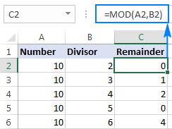
3 things you should know about MOD in Excel
- The result of the MOD function has the same sign as the divisor.
- If the divisor is 0, MOD returns the #DIV/0! error because you cannot divide by zero.
- If the number or divisor is a text value, an Excel Mod formula returns the #VALUE! error.
MOD formulas to calculate cells
In real-life worksheets, the Excel MOD function is rarely used on its own. More often, you will find it as part of bigger formulas that perform various calculations based on division remainder.
Mod formula to sum every Nth row or column
Surprising at it may seem, Microsoft Excel has no built-in function to sum every 2nd, 3rd, etc. row in a worksheet. However, that can be easily done by using one of the following formulas.
Sum every other row
To add up values in every second row, use MOD in conjunction with ROW and SUMPRODUCT:
Sum even rows:
Sum odd rows:
Assuming B2:B7 are the cells to sum, the formulas look as follows:
Sum even rows:
=SUMPRODUCT((MOD(ROW($B$2:$B$7),2)=0)*($B$2:$B$7))
Sum odd rows:
=SUMPRODUCT((MOD(ROW($B$2:$B$7),2)=1)*($B$2:$B$7))
The screenshot below shows the result:
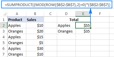
In these formulas, the MOD ROW combination determines which rows to sum and SUMPRODUCT adds up the values. Here's how:
ROW supplies an array of row numbers to the number argument of the MOD function. MOD divides each row number by 2, and you check the result:
- To sum even rows, the result should be 0 because even numbers are divisible by 2 evenly, without remainder.
- To sum odd rows, the result should be 1 because odd numbers divided by 2 leave a remainder of 1.
Instead of SUMPRODUCT, you could use the IF function to evaluate the condition and SUM to add up the numbers (it's an array formula, which is entered by pressing Ctrl + Shift + Enter):
=SUM(IF(MOD(ROW($B$2:$B$7),2)=0,$B$2:$B$7,0))
Personally, I'd stick with SUMPRODUCT because ROW is a volatile function and using it in an array formula makes the whole formula volatile. That means the formula would recalculate with every change you make to a workbook, which may noticeably slow down your Excel.
Sum every Nth row
To add up every 3rd, 4th, 5th, etc. row, use this generic formula:
For example, to sum every 3rd cell in the range C2:C10, the formula goes as follows:
=SUMPRODUCT((MOD(ROW($C$2:$C$10)-ROW($C$2)+1,3)=0)*($C$2:$C$10))
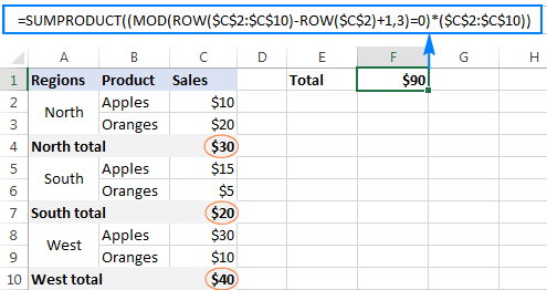
Compared to the previous example, this formula has a bit more complex "filtering logic":
MOD(ROW($C$2:$C$10)-ROW($C$2)+1,3)=0
First, you subtract the first row from all other rows in the range to get an array of relative row numbers {0;1;2;3;4;5;6;7;8}, to which you add 1 to start counting from one: {1;2;3;4;5;6;7;8;9}
The above array goes into the number argument of the MOD function, which returns the remainder after dividing each number by 3: {1;2;0;1;2;0;1;2;0}
Note that zeros appear for every 3rd row, and MOD()=0 tells Excel to return TRUE only for these rows, FALSE for all other rows. With TRUE equating to 1 and FALSE to 0, we are left with an array of {0,0,1,0,0,1,0,0,1}
Finally, SUMPRODUCT multiplies the above array and C2:C10, and then adds up the products. Since multiplying by zero always gives 0, only the rows that contain 1 in the first array survive the multiplication.
Sum every Nth column
To sum numbers in every 2nd, 3rd, etc. column, simply replace ROW with COLUMN in the above formula, like this:
For example, to add up numbers in every 4th column in the range B2:I2, you go with this formula:
=SUMPRODUCT((MOD(COLUMN($B2:$I2)-COLUMN($B2)+1,4)=0)*($B2:$I2))

Mod formula to concatenate every N cells
In situations when the details relating to the same item are split into several cells, combining the contents of every N number of cells into one cell may be a challenge.
In this example, we have order details in three different cells in column B, so we are looking to concatenate each block of three cells, beginning with B2. This can be done with the following formula:
=IF(MOD(ROW()-1, 3)=0, CONCATENATE(B2, "-", B3, "-", B4), "")
Important note! For the formula to work correctly, it shall be entered in the 3rd row with data (C4 in this example), and then copied down the column.
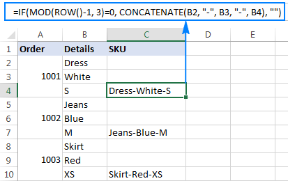
The formula's logic is very simple:
First, you check if a given row is divisible by 3 with no remainder: MOD(ROW()-1, 3)=0. To get the relative position of the current row, we subtract 1 from the actual row number (since our data begins in row 2, not in row 1). If the division remainder is equal to 0, the CONCATENATE function combines values from 3 cells and separates them with the delimiter of your choosing ("-" in this example). The use of relative cell references ensures that three different cells are concatenated each time.
Tip. Instead of the -1 correction, you can get the relative position of each row as we did in the above example, i.e. IF(MOD(ROW()-ROW($B$2)+1, 3)=0, CONCATENATE(), "")
This will make your formula more flexible and it won't require further adjustments no matter in which row your data starts.
Mod formulas to count cells that contain odd or even numbers
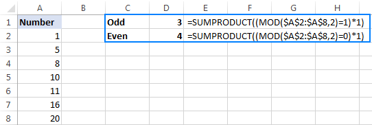
As you already know, the easiest way to identify an even integer is divide the number by 2 and check for zero remainder. To identify an odd number, you check for a remainder of 1. Again, we will be using the MOD function to find remainders, and SUMPRODUCT to count the "filtered cells".
Count cells with odd numbers:
Count cells with even numbers:
With numbers in cells A2 to A8, the formulas take the following shape:
Count cells containing odd numbers:
=SUMPRODUCT((MOD(A2:A8,2)=1)*1)
Count cells containing even numbers:
=SUMPRODUCT((MOD(A2:A8,2)=0)*1)
How to use MOD in Excel to highlight cells
Aside from calculating cells based on a specific remainder, the MOD function in Excel can be used to highlight those cells. For this, you will have to create a formula-based conditional formatting rule. The detailed steps to set up a rule can be found here, and the formulas are provided below.
Highlight odd and even numbers
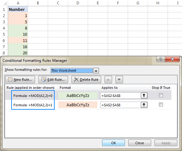
To highlight cells containing odd or even numbers, use the following Excel Mod formula that divides the number by 2, and then checks for a remainder of 1 and 0, respectively:
Highlight cells with odd numbers:
=MOD(A2,2)=1
Highlight cells with even numbers:
=MOD(A2,2)=0
Where A2 is the leftmost cell with data.
Highlight integers and decimals
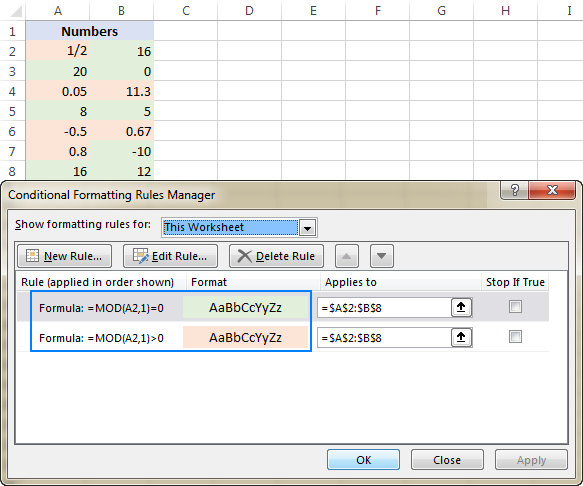
To identify integers, just follow this logical chain: any number divided by 1 equals itself, meaning an integer divided by 1 is always the same integer, meaning the remainder is zero, meaning we can use this simple MOD formula:
=MOD(A2,1)=0
If the remainder is greater than zero, you are dealing with a fraction (including decimals):
=MOD(A2,1)>0
Since in formula-based conditional formatting rules cell references are relative to the top left cell of the selected range, we reference A2 in this example:
Highlight multiples of a number
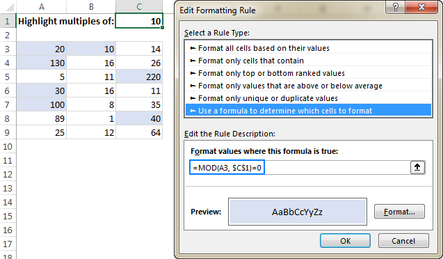
To highlight multiples of a specific value, simply divide a number by that value and check for zero remainder.
For example, to highlight cells containing 10 and all its multiples, use this formula:
=MOD(A3,10)=0
Where A3 is the top left cell in the range for which you create the rule (A3:C9 in the screenshot below).
Or, you can input the number of interest in any empty cell, say C1, and reference that cell in your formula (remember to lock the cell with an absolute reference):
=MOD(A3, $C$1)=0
Excel MOD with Data Validation
Another clever use of the Excel MOD function can be preventing entry of certain data in selected cells, such as odd numbers, even numbers, or decimals. This can be done with the same MOD formulas that we've used to highlight cells, but this time we will be defining a Data Validation rule.
To make a data validation rule based on a formula, click Data > Data Validation. On the Settings tab, select Custom in the Allow box, and enter your formula in the Formula box. For the detailed steps, please see How to create a custom validation rule in Excel.
For example, to allow only integers in cells A2:A8, select these cells, and configure a rule with this formula:
=MOD(A2,1)=0
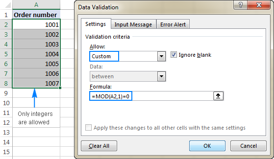
In a similar fashion, you can limit the data entry to even or odd numbers:
Allow only odd numbers:
=MOD(A2,2)=1
Allow only even numbers:
=MOD(A2,2)=0
Where A2 is the left-top-most cell of the selected range.
That's how you use the MOD function in Excel to find the division remainder and perform other calculations. To have a closer look at the formulas discussed in this tutorial, you are welcome to download our sample Excel MOD workbook. For more formula examples, please check out the resources at the end of this page.
I thank you for reading and hope to see you on our blog next week!
 by
by
24 comments
I would like to have all the text in a row turn to red when the word 'Expense' is chosen from drop down list in a cell in the same row. What would the MOD formula be to achieve this for the whole table please?
Hello Lee!
The MOD function is used to work with numbers, not text.
If I understand your task correctly, to change a row's color by condition, use conditional formatting. This article may be helpful: Change the row color based on cell value.
I've found the following answer since posting my own question:
In Conditional Formatting, select 'Use a formula to determine which cells to format' and enter =$B1="Expense"
So this does not need to be a MOD formula.
Bonjour
Je cherche a faire commencer mon tableau de bilan en septembre et non janvier
=SUMPRODUCT((MONTH(Recettes!$A$4:$A$200)=1+COLumn()-3)*(Recettes!$C$4:$C$200='Synthèse'!$A9)*(Recettes!$E$4:$E$200))
j'ai tenté mais sans succes
=SUMPRODUCT((MONTH(Recettes!$A$4:$A$200)=MOD(7+COLUMN()-COLUMN($C$1),12)+1)*(Recettes!$E$4:$E$200))
Hello Eric!
Without seeing your data and without any explanation of your formula, it is impossible to understand it and give advice.
Is there an excel formula to find a divisor when dividend and the quotient are cells A1 and C1 in a worksheet?
In other words, I want to solve for X, when A3 ÷ X = C3.
Thank you for your help!
Robert Garber
Hi! It's just math. X=A3/C3
Hi.
I have a column A with value 214.
In column B I have A1/13 which gives me 18.54.
What formula can I use to show 18 and a 7 for the remainder instead of .54
Thanks
Hi! If I understand your task correctly, the following formula should work for you:
=IF(MOD(B1,1)<0.7,INT(B1)+0.7,B1)
You can learn more about INT function in Excel in this article on our blog.
I am trying to find a formula using the MOD formula, maybe a nested if function to make a integer whole that is divisible 3. The values have different remainders. Trying to get the remainder to 0.
Values divisible by 3: 8, 6, 20, 1153, 536, 1
Remainder: 1, 2
End result for remainder using formula; would like to see 0
Hi! What does the “Values divisible by 3: 8” phrase mean? It's incorrect. What result do you want to get exactly?
Thank you for replying, Alexander. Let me clarify a bit. I have random units value that need to be divisible by 3 only. Ideally I want all remainder units value to equal 0. For example I can get different remainders, i.e. 1, 2, 3 e.t.c. when I divide by 3. Can’t figure out the formula that would tell me which way I should round on the units up or down to get the remainder to 0 when divisible by three.
Hi! Depending on the result of the MOD formula, use the CHOOSE function to select which number to add to the original value.
=A1+CHOOSE(MOD(A1,3)+1,0,-1,1)
For more information, read: CHOOSE function in Excel with formula examples.
Thank you, Alexander. This is very helpful and is saving me 20 mins from this task. Super appreciated.
What formula can I use if I am dividing a number by 2 but I want to add a +1 if it returns an even number and rounds up if it returns an odd number? For example, if the number is 19 then 19/2 yields a 9.5 and then rounding it up makes 10. Conversely, if I had 10, then 10/2 returns 5 and then I want to add 1 to make it 6.
Hi! To define an even number, use the MOD function. I don't know how you want to round, but here is a sample formula:
=IF(MOD(A2,2)=0,A2/2+1,ROUND(A2,0))
Thank you very much for all your efforts and the help that you provide. It's simply beyond any price!!
Hello 🙂
I have a table where I was to calculate every other columns value at the end of each row,
for example; B2, D2, F2, H2, J2, and so on. Extra columns will get added so I'm hoping the formula works to take that into account...?
I potentially could flip the table so I'd be calculating every other row instead if that works better but I'd rather not.
I've spent hours researching and trying different formulas and keep getting things like;
'The range {insert attempted range here} can’t be used as a single value.'
and
'The formula uses a Boolean in place of a number.'
Any help would be hugely appreciated.
Thanks
Hello!
If you want to find the last value in a row in Excel, you can use the INDEX MATCH function. Formula example:
=INDEX(1:1, MATCH(9.99E+307, 1:1))
This formula will return the last value in row 1.
Please note that if there are empty cells in the row, then this formula will return the value of the last filled cell. If you need to find the last cell in a row, including empty cells, use the following LOOKUP formula:
=LOOKUP(2,1/(1:1<>""),1:1)
I hope it’ll be helpful.
Please solve the equation {=mod(50,-7) =-6}.... How it come explain me please
7 goes into 50 8 times (56) remainder -6 = 50. The rule is that the mod has to be the same sign as the divisor, in this case negative forcing you to overshoot the multiple by one so that the negative remainder can bring you back to the dividend, in this case 50.
Hello!
Sorry, I do not fully understand the task. For me to be able to help you better, please describe your task in more detail. Please specify what you were trying to find, what formula you used and what problem or error occurred. Give an example of the source data and the expected result.
It’ll help me understand it better and find a solution for you.
Thank you so much,
Very good explanation on MOD.
the formula Mod((sqrt(n)*180)-225,360) calculates degrees of any number on a circle starting on the horizontal left as zero going clock wise.
How would you modify the above Mod formula to calculate degrees of any number if the zero was placed on the horizontal right and was moving counter
clock wise?