This short tutorial explains different ways to add, use and remove strikethrough format in Excel desktop, Excel Online and Excel for Mac.
Excel is great for manipulating numbers, but it does not always make clear how to format text values the way you want. Strikethrough is a vivid example.
It is super easy to cross out text in Microsoft Word - you simply click the strikethrough button ![]() on the ribbon. Naturally, you'd expect to see the same button on the Excel ribbon. But it's nowhere to be found. So, how do I strikethrough text in Excel? By using any of the six methods described in this tutorial :)
on the ribbon. Naturally, you'd expect to see the same button on the Excel ribbon. But it's nowhere to be found. So, how do I strikethrough text in Excel? By using any of the six methods described in this tutorial :)
How to strikethrough in Excel
To ensure that everyone is on the same page, let's define the term first. What does it mean to strikethrough in Excel? Simply, to put a line through a value in a cell. There are a handful of different ways to do this, and we are going to begin with the fastest one.
Excel strikethrough shortcut
Want to have the job done as quickly as possible? Press a hotkey or key combination.
Here's the keyboard shortcut to strikethrough in Excel: Ctrl + 5
The shortcut can be used on an entire cell, certain part of the cell contents, or a range of cells.
To apply the strikethrough format to a cell, select that cell, and press the shortcut:

To draw a line through all values in a range, select the range:

To strikethrough non-adjacent cells, select multiple cells while holding the Ctrl key, and then press the strikethrough shortcut:

To cross out part of the cell value, double-click the cell to enter the Edit mode, and select the text you want to strikethrough:

Apply strikethrough via cell format options
Another quick way to draw a line through a cell value in Excel is by using the Format Cells dialog. Here's how:
- Select one or more cells on which you want to apply the strikethrough format.
- Press Ctrl + 1 or right-click the selected cell(s) and choose Format Cells… from the context menu.
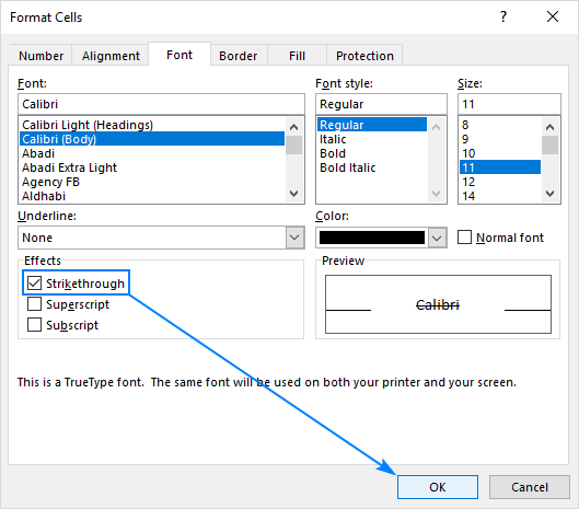
- In the Format Cells dialog box, go to the Font tab, and tick off the Strikethrough option under Effects.
- Click OK to save the change and close the dialog.
Add a strikethrough button to Quick Access Toolbar
If you think that the above method requires too many steps, add the strikethrough button to the Quick Access Toolbar to always have it at your fingertips.
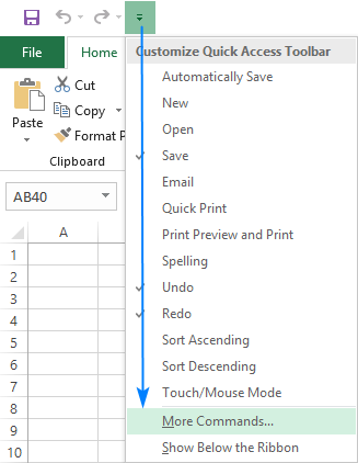
- Click the small arrow in the upper left corner of the Excel window, and then click More Commands…
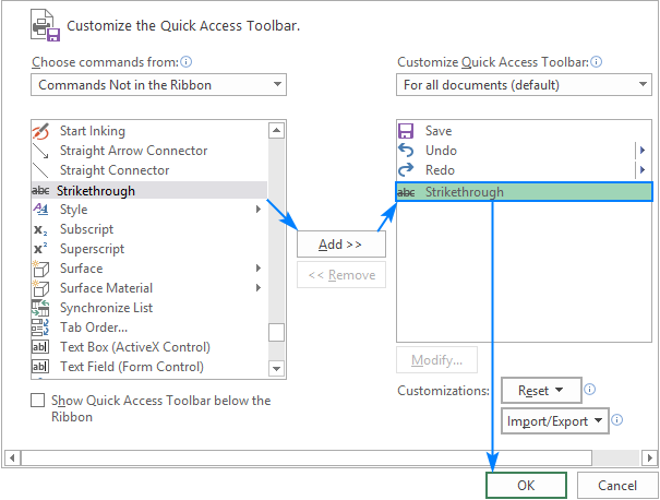
- Under Choose commands from, select Commands Not in the Ribbon, then select Strikethrough in the list of commands, and click the Add button. This will add Strikethrough to the list of commands on the right pane, and you click OK:
Look at the upper left corner of your worksheet again, and you will find the new button there:
![]()
Put a strikethrough button onto Excel ribbon
If your Quick Access Toolbar is reserved only for the most frequently used commands, which strikethrough is not, place it onto the ribbon instead. As with QAT, it's also one-time setup, performed in this way:
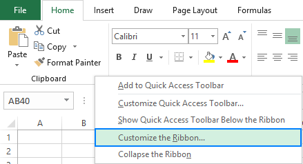
- Right-click anywhere on the ribbon and select Customize the Ribbon… from the pop-up menu:
- Since new buttons can only be added to custom groups, let's create one. For this, select the target tab (Home in our case) and click the New Group button. Then, click Rename… to name the newly created group to your liking, say My Formats:

- With the new group selected, perform the already familiar steps: under Choose commands from, select Commands Not in the Ribbon, find Strikethrough in the list of commands, select it, and click Add:
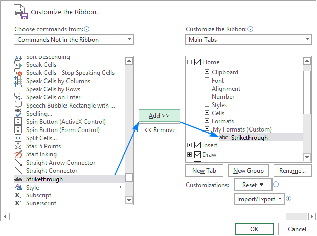
- Click OK to save the changes, and find the Strikethrough button on your Excel ribbon:

You can now cross out text in Excel with a single button click! And it will also remind you the keyboard shortcut in case you forget it :)
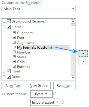
Tip. By using Up and Down arrows in the Excel Options dialog box, you can move your custom group with the Strikethrough button to any position on the ribbon:
How to strikethrough automatically with conditional formatting
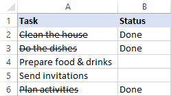
In case you are planning to use a strikethrough to cross out the completed tasks or activities in a checklist or to-do list, you may want Excel to do it for you automatically as you enter some text in a related cell, for example "done":
The task can be easily accomplished with Excel Conditional Formatting:
- Select all the cells you want to cross out on condition (A2:A6 in this example).
- On the Home tab, in the Styles group, click Conditional Formatting > New Rule…
- In the New Formatting Rule dialog box, select Use a formula to determine which cells to format.
- In the Format values where this formula is true box, enter the formula that expresses the condition for your topmost cell:
=$B2="Done" - Click the Format…
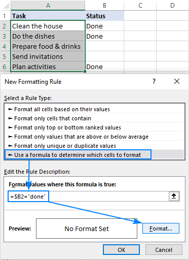
- In the Format Cells dialog box, switch to the Font tab and select the Strikethrough Optionally, you can make some other formatting changes, e.g. set a light grey font color for crossed out entries:
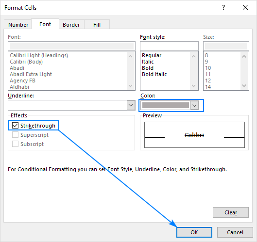
- Click OK to close the Format Cells dialog box, then click OK one more time to close the New Formatting Rule window, and you are all set!

Instead of defining a task status with text, you can insert checkboxes, link them to some cells (which you can hide later) and base your conditional formatting rule on the value in the linked cells (TRUE is a checkbox is checked, FALSE if not checked).
As the result, Excel will check off the completed tasks automatically depending on whether the checkbox is selected or not.

If you'd like to create something similar in your worksheets, the detailed steps can be found here: How to create a checklist with conditional formatting.
Add strikethrough with a macro
If you are not allergic to using VBA in your Excel worksheets, you can apply strikethrough on all selected cells with this line of code:
The step-by-step instructions on how to insert VBA code in Excel can be found here.
How to use strikethrough in Excel Online
In Excel Online, the strikethrough option is exactly where you'd expect to find it - next to the other formatting buttons on the Home tab, in the Font group:
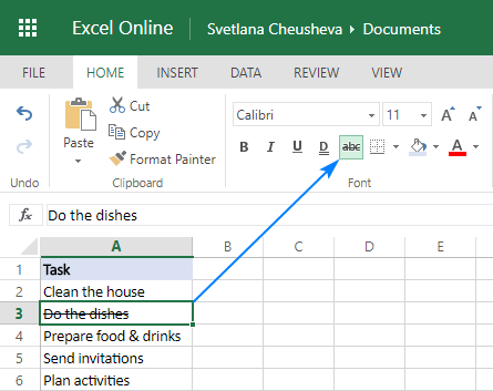
However, there's a fly in the ointment - it's not possible to select non-adjacent cells or ranges in Excel Online. So, if you need to cross out multiple entries in different parts of your sheet, you will have to select each cell or a range of contiguous cells individually, and then click the strikethrough button.
The strikethrough shortcut (Ctrl + 5) works perfectly in Excel Online too and is often the fastest way to toggle the strikethrough formatting on and off.
In case you are interested, you can learn more about how to move your worksheets in Excel Online.
How to strikethrough in Excel for Mac
A quick way to strikethrough text in Excel for Mac is by using this keyboard shortcut: ⌘ + SHIFT + X

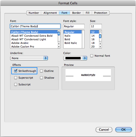
It can also be done from the Format Cells dialog in the same way as in Excel for Windows:
- Select the cell(s) or part of a cell value you wish to cross out.
- Right-click the selection and chose Format Cells from the popup menu.
- In the Format Cells dialog box, switch to the Font tab and select the Strikethrough checkbox:
How to remove strikethrough in Excel
The correct way to remove strikethrough from a cell depends on how you've added it.
Remove strikethrough added manually
If you applied strikethrough via a shortcut or cell format, then press Ctrl + 5 again, and the formatting will be gone.
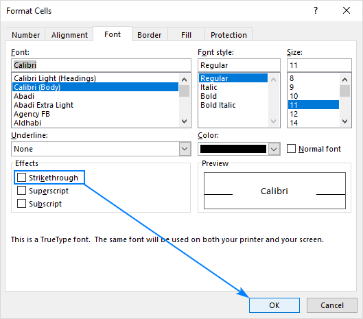
A longer way would be opening the Format Cells dialog (Ctrl + 1) and unchecking the Strikethrough box there:
Remove strikethrough added with conditional formatting
If strikethrough is added by a conditional formatting rule, then you need to remove that rule to get rid of strikethrough.
To have it done, select all the cells from which you want to remove strikethrough, go to the Home tab > Styles group, and click Conditional Formatting > Clear Rules > Clear Rules from Selected Cells:
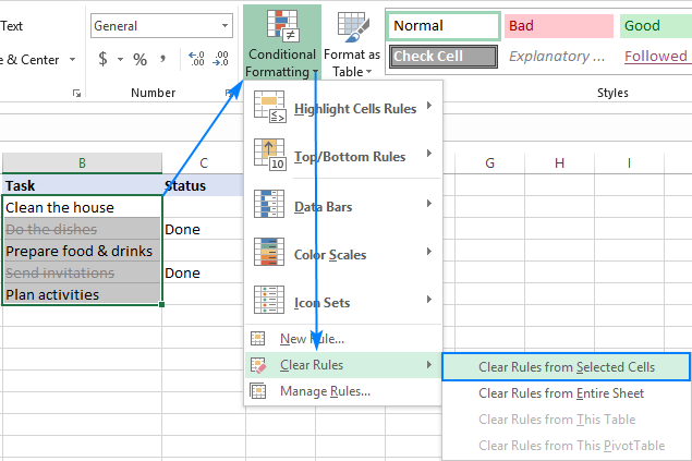
If some other conditional formatting rule(s) is applied to the same cells and you'd like to keep that rule, then click conditional Formatting > Manage Rules… and delete only the strikethrough rule.
For more information, please see How to delete conditional formatting rules in Excel.
That's how you can add and remove the strikethrough formatting in Excel. I thank you for reading and hope to see you on our blog next week!
 by
by
28 comments
Is there any option to strikethrough the "Sheet Name"???
Thank you so much! Very useful!
Is there a way of striking out in a different colour to the text colour?
Thanks,
Thanks for the tips. Very precise. Good job!
Thank you!
thank u..very helpful..
ITS VERY HELP FULL TO US THANK U
This was very comprehensive and helpful. Thank you!
Is there a way to add a column of strike through buttons for each row to allow me to check and uncheck rows quickly?
I just wanted to leave a quick but MASSIVE THANK YOU!! I've been searching for literal hours trying to find something that would help me do JUST what your article helps me do, and yet the amount of complications I had to go through, and it not working out, was downright frustrating.
Your instruction were very clear and easy to follow. Thank you again!
Hello - I'm working in a table, with data validation list drop downs. When I use the conditional formatting to strike out an entire row, it formats the row below the row I want to strike out. Why would that be?
Hello Ann!
Unfortunately, without seeing your data it hard to give you advice. For me to be able to help you better, please describe your task in more detail. Please specify what formula you used and what problem or error occurred. It’ll help me understand it better and find a solution for you. Thank you.
Thank you very useful!
Thanks so much for your sharing. This is very informative and helpful.
I've learned that the conditional formatting can be done with this Excel VBA code:
Private Sub ConditionalFormatting1()

    Dim Target As Range

    Target = Columns("A")

    Target.FormatConditions.Delete

    Target.FormatConditions.Add _

        Type:=xlExpression, _

        Formula1:="= $B1 = ""Done"" "

    With Target.FormatConditions(1).Font

        .Strikethrough = True

        .ThemeColor = 10

    End With

End Sub
Hi there,
Could you please help me with my issue: I have A1 cell which has text file let's say: "This is my issue". Some of the words are strikethrough: is and issue. In A2 I have the formula which is simple: "=A1". With this I receive the full text in A1, but the 2 strikethrough words are normal, without the formating. Would be somehow possible to copy/link the formatting part as well? Thank you!
Hello!
Formatting part of the text in a cell is only possible manually
Awesome! Thank you for your sharing! :)
try to build the solid foundation of the bricks that others have taken, life will not be so hard.
How do I make the strike-through line thicker?
I doubt that it's possible to change the thickness of a strikethrough line, even with VBA.
Very helpful !
Ctrl-5 to Strikethrough!? Magical!
This is very informative and helpful. Thank you!
the mac shortcut is wrong
Hi Alison,
Oops, you are right. The second key was wrong. Here's the correct strikethrough shortcut for Mac: Command + Shift + X. Fixed, thank you!