How to do a vlookup without errors in Google Sheets? Take a closer look at the most common mistakes made when working with the VLOOKUP function.
Google Sheets VLOOKUP is one of the most useful yet trickiest functions. It helps finding matching data across multiple sheets. However, there are cases when your formula may return errors like #N/A, #NAME?, #VALUE!, or #REF!.
Let's try and answer the following question together, "Why my Google Sheets VLOOKUP isn't working?"
Most common VLOOKUP mistakes
The first reason is that there are simply no matches in the range you indicated. You're powerless here and can't affect the result.
Other cases mean that you've made a mistake somewhere in the formula. Let's take a closer look at what may have gone wrong.
Wrong delimiters
Delimiters are those characters that are used in formulas as separators. For example, if you are in the UK or the US, chances are your formulas require commas as delimiters:
=VLOOKUP(A2,$F$2:$G$10,2,FALSE)
And it is your spreadsheet locale that controls the separator choice. Different locales call for different separators.
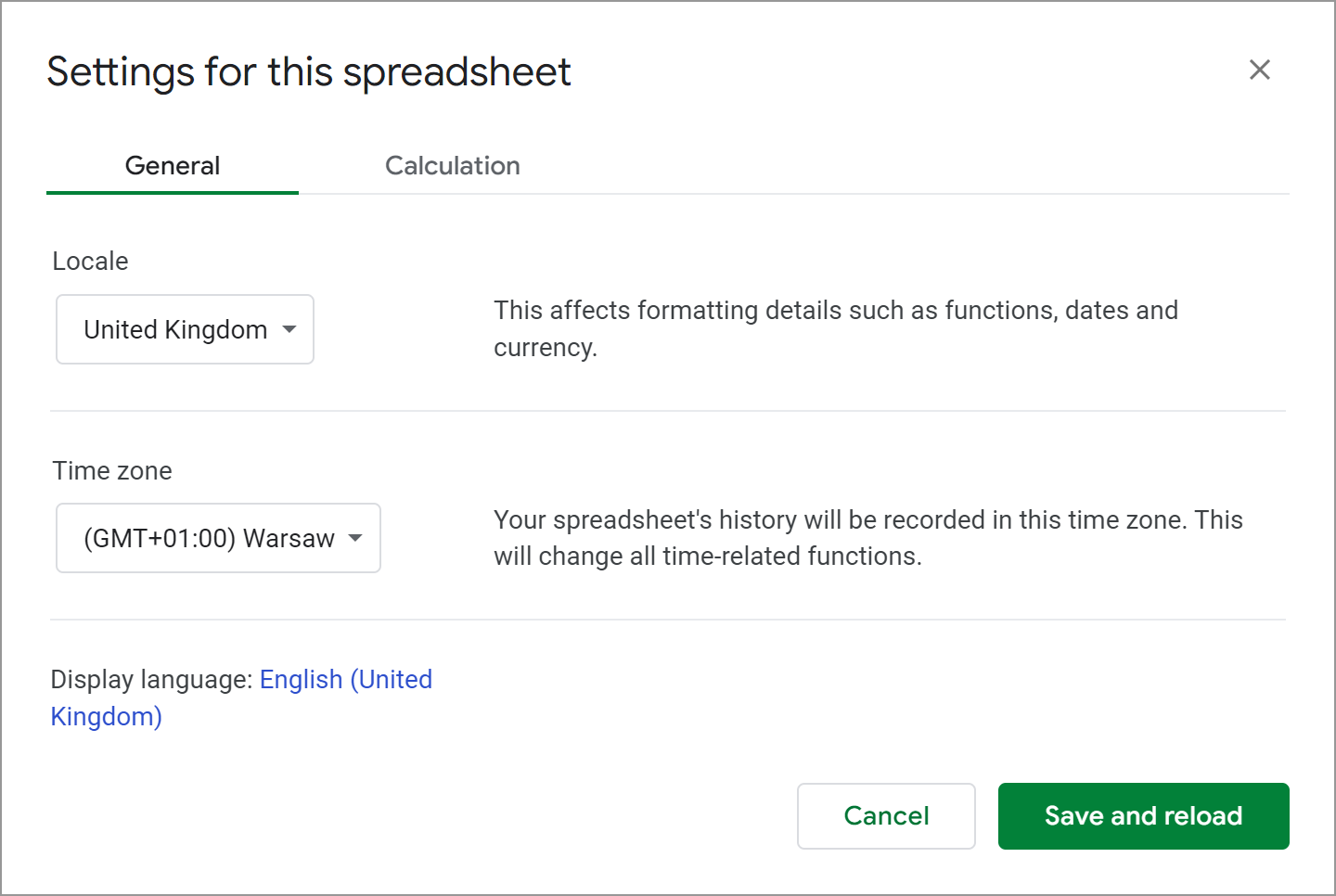
To check your locale in Google Sheets, go to File > Settings. You'll see the locale under the General tab:
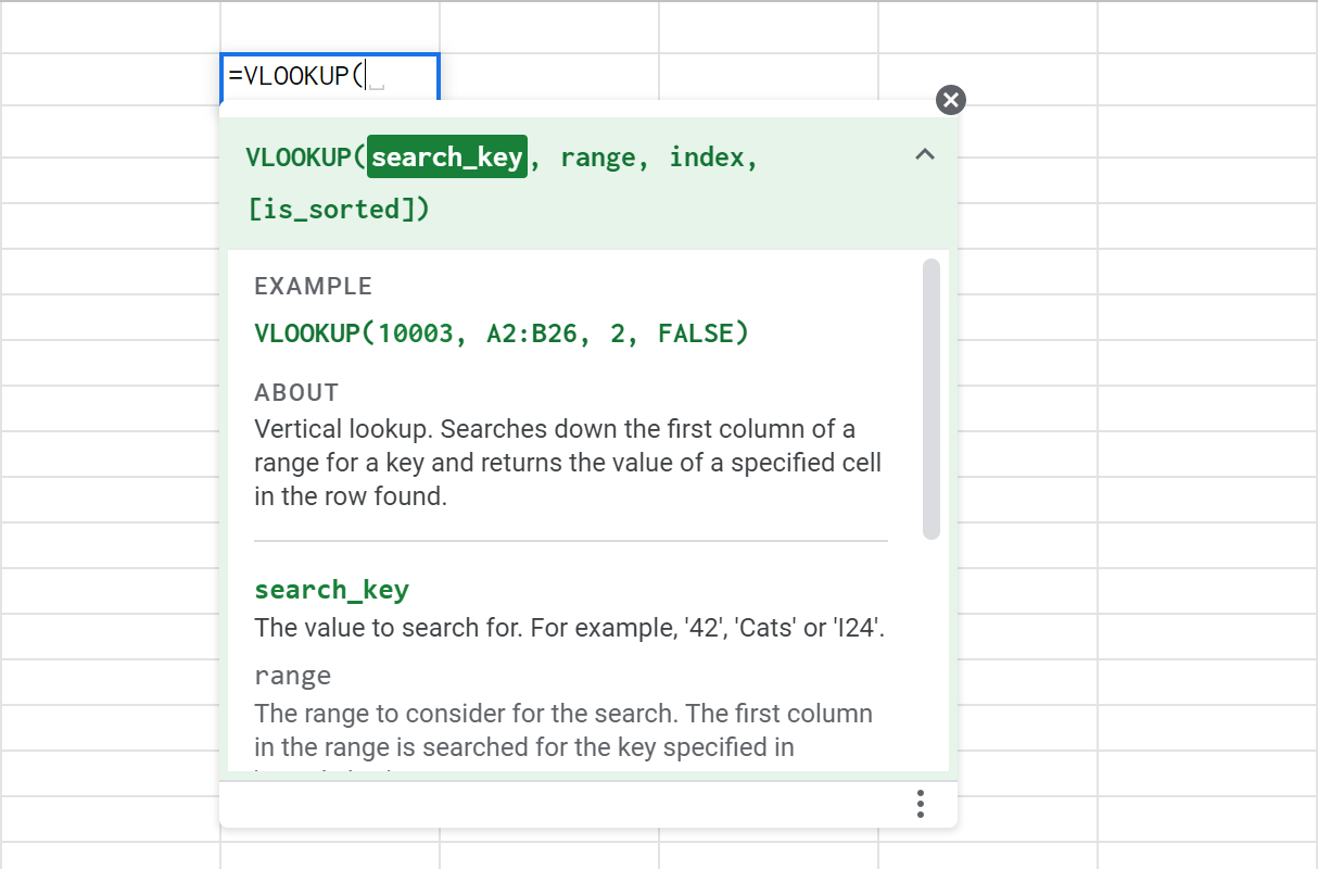
To understand what delimiters your VLOOKUP needs based on your locale, just start entering the function. Google Sheets will show you what your formula should look like exactly and what separators must be used:
If the delimiters are all correct but your Google Sheets VLOOKUP still fires errors, check other possible issues and their solutions below.
Incorrect data – #N/A error
The formula can't find anything and returns the #N/A error? But you're sure there's got to be a match?
The simplest solution is the best here – most likely, you entered the data into the formula incorrectly. This may happen especially if you type the formula directly into the formula bar rather than the cell.
Fix this #N/A error
Double-check all arguments, make sure all cell references and values are correct.
Or add your own text for when there's really no match.
Incorrect function name – #NAME? error
If you see the #NAME? error, you either wrote the function name incorrectly (missed or misspelled a letter or two) or got mixed up with the syntax.
Fix the #NAME? error
Check the function name and the VLOOKUP syntax. Correct all the typos, and everything will work.
Invalid VLOOKUP cell references – #N/A error
The formula worked just fine until you added a few rows or columns into the table and the #N/A error appeared out of the blue?
Fix this #N/A error
Check if the search range and the cell with the value to look for are entered correctly – they are neither misspelled nor absent from the sheet.
Note. If you use relative cell references (e.g. A1) instead of absolute ones (e.g. $A$1) and then modify the table (e.g. add a column), the data will shift, the references will change, and the formula will refer to wrong cells:
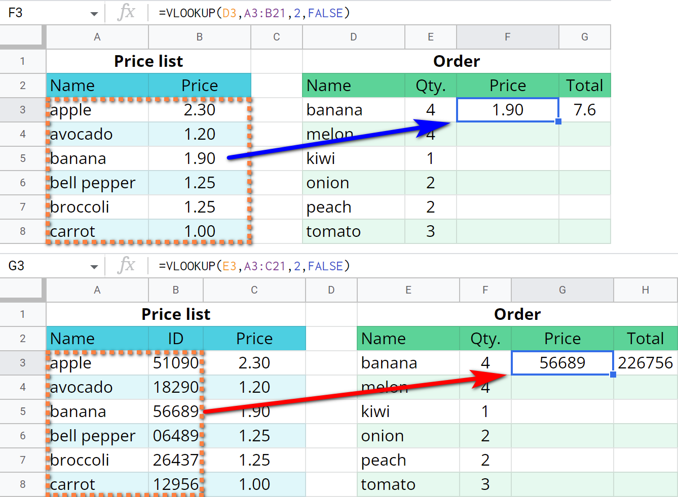
I added the "ID" column. The "Price" column is not included in the range anymore, thus the price cannot be found.
If that happens, simply Undo the table modifications and fix the references.
Incorrect "is_sorted" argument
Your Google Sheets VLOOKUP formula is set to return approximate match (TRUE) while the lookup column is not sorted.
To fix that, either sort data by the lookup column A to Z or change TRUE to FALSE.
Incorrect lookup range – #N/A error
You may have forgotten that the VLOOKUP function in Google Sheets always searches in the first (leftmost) column of the lookup range. If the values for the search_key argument are in the second or some other column, VLOOKUP won't work and will return the #N/A error:
Note. Remember: VLOOKUP cannot look at its left. With that in mind, adjust your table or the formula. Or use INDEX/MATCH instead.
Fix this #N/A error
Incorrect column number – #VALUE! error
Sometimes the third argument of Google Sheets VLOOKUP is indicated incorrectly.
It cannot be less than 1 and more than the total number of columns in the search range. If the number is incorrect, VLOOKUP in Google Sheets will return the #VALUE! error.
Note. The number of the column should be 1 or more. Of course, it's unlikely that you'll enter 0 or -1, but if you use some other functions to get the serial number of the required column, you may stumble upon the error.
Fix the #VALUE! error
If that happens, please count the number of columns in the entered range and make sure it includes the number from the third argument of the VLOOKUP function.
Invalid reference to another table – #REF! error
The search range can be in another table or even another Google spreadsheet.
You'll notice that something's off if you see the #REF! error.
It means that the range you put into the formula is invalid and the function cannot locate it.
Incorrect Number format – #N/A error
This means that the format of the cell with a required value (D3 in our case) and the format of the leftmost column in the search range (A3:A21 in our case) differ (numeric and textual).
This may happen when you use numeric codes instead of textual entries (order numbers, goods IDs, dates, and other identifiers).

As the example above shows, the values look the same but the entry in D6 is formatted as a number while A10 contains a text string. The text cannot be treated as a number, making the VLOOKUP function in F6 return the #N/A error in Google Sheets.
Fix this #N/A error – change the format
If there's only one error like this, you can swiftly fix it by changing the cell's number format. Select the cell and go to Format > Number > Plain text in the Google Sheets menu. Its contents will be changed into the text:

Do that, and the error will be gone since you'll be looking for the text string among other text strings.
Fix this #N/A error – use the TEXT function
Alternatively, you can add the TEXT function that will transform any values into text.
I use the following formula:
=VLOOKUP(TEXT(D6,"#"),$A$3:$B$21,2,FALSE)
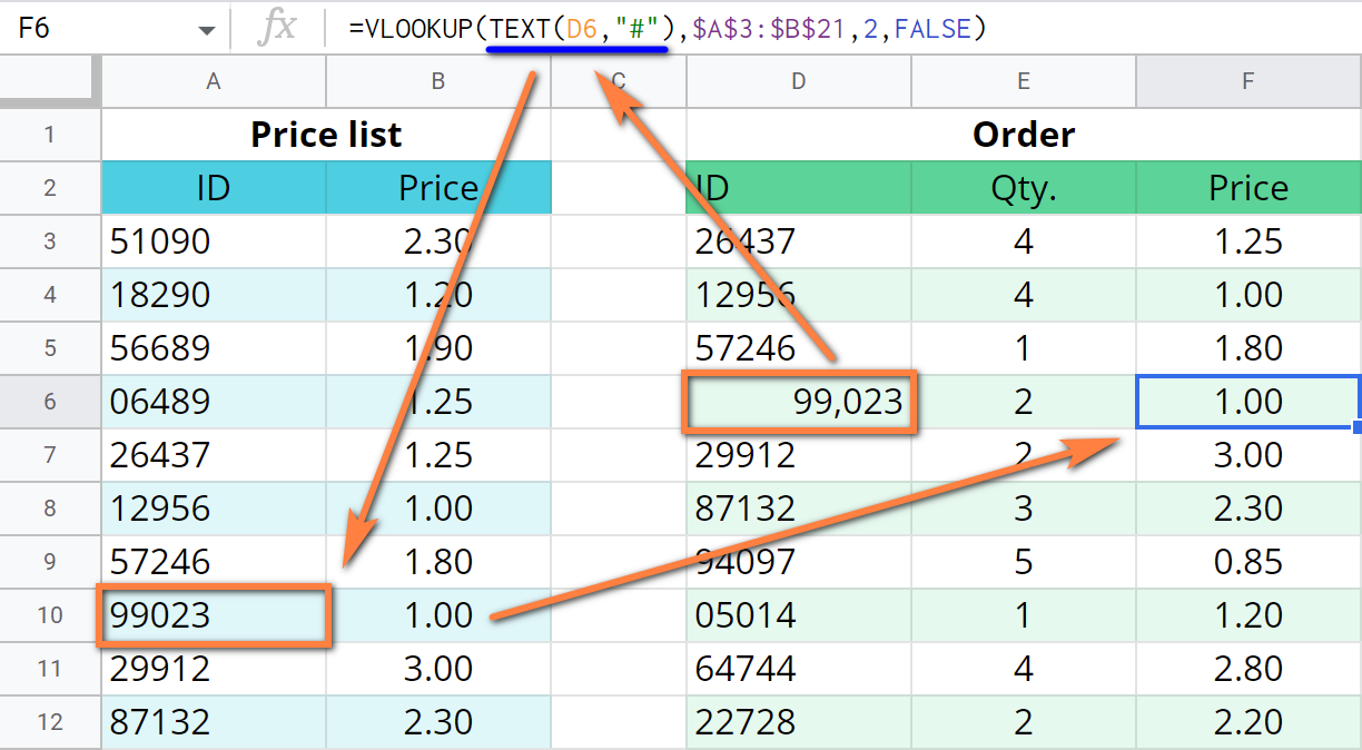
I replaced the usual cell reference to D6 with another function:
TEXT(D6,"#")
The arguments of the TEXT function are very simple:
- The first argument, number, indicates the cell to format.
- The second argument, format, is a pattern to which I'm going to convert the value of the cell.
Excess spaces and non-printing characters – #N/A error
The function is unable to find the required value since the cell contains excess spaces or non-printing chars (line breaks and others).
In my example, Google Sheets VLOOKUP is not working because there are two trailing spaces typed into D4 accidentally. And since the function compares symbols, the search fails:

This problem is quite common and invisible to the eye. For example, if the value consists of two words, an excess space may find its way in between the words.
You may also accidentally enter such non-printing characters that are hidden on the screen (tabulations, line breaks, etc).
Fix this #N/A error – use TRIM and CLEAN functions
The TRIM and CLEAN functions that are designed for text strings will help and remove unwanted invisible characters:
=VLOOKUP(TRIM(CLEAN(D4)),$A$3:$B$21,2,FALSE)
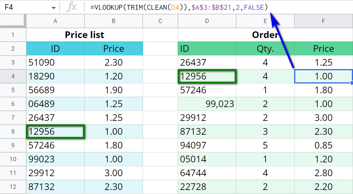
The TRIM function removes extra spaces while the CLEAN function deletes all non-printing characters.
Tip. You can always use this combination of functions "just in case" to avoid any errors.
Fix this #N/A error – use a special tool to trim spaces
Or use the Remove tool from Power Tools to delete all unwanted characters at once:

Install Power Tools to your Google Sheets to remove all unwanted characters in one go.
Replace VLOOKUP errors with your own text
I think you will agree that errors don't make your table look good. Is there a way to get rid of them?
Well, yes, but it won't hurt to first double-check if your VLOOKUP formula in Google Sheets was built correctly:
- Start with the lookup range. Did you put it correctly? Does your value appear in the leftmost columns of this range?
- Make sure the "is_sorted" argument is correct: TRUE or FALSE, depending on the match you need and the sorting of your range.
- Check for all possible number formats mismatches and extra spaces or non-printing chars.
Tip. Avoid using VLOOKUP errors by switching to other more powerful ways of fetching the data.
If everything looks fine yet the formula doesn't return the value, add the IFERROR function there:
=IFERROR(VLOOKUP(D9,$A$3:$B$21,2,FALSE),"No match")
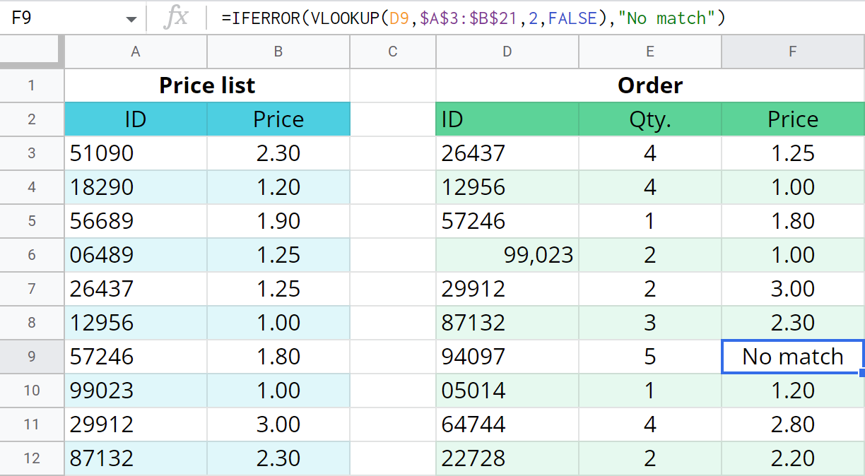
The syntax of IFERROR is easy to understand:
- value – something we check for errors. If everything's fine, the result of our calculation returns.
- [value_if_error] – something the function returns if the first argument catches an error.
In my case, F9 shows "No match" because VLOOKUP can't find any matches.
This is how you check your VLOOKUP function for errors in Google Sheets. If you double-check all these but your formula still won't work, let us know in the comments sections below.
 by
by 
39 comments
Thank you for this. This is a nice detailed manual. Thank you for doing this for us
Thank you for your feedback, André! We're glad the article could help! :)
Hi everybody,
My error is not listed here, i don't know if its an error or something else. I tried to find my payments of monthly orders with order Ids, but instead of numbers its shows different dates for different order Ids. For example if the order ID is 'OD327424530139374100', the result it shows is 'Sep 17, 1901' and so on..
Can anyone help me understand the problem and fix it??
Thanks.
Hi Ramiz Anjum Lasar,
It looks like your cells are formatted as dates. Select them, go to Format > Number format and pick the correct format: number, text, or try automatic.
Sometime flipping columns appears to resolve the issue - Say return result is in Column 1 and and look up value in Column 2 - then move column to 1 and make it column 2 and vice versa.
Hello Gary,
Thank you for the tip. Is it for when VLOOKUP cannot look at its left?
I found a Bug?
https://docs.google.com/spreadsheets/d/1Wrmhmbz2YumspRd_qXuLNwcS-cjXZW6ZgjWkkxJTr68
You can see 2 pages, on the first page the VLOOKUP is not working, and in the second page is working! I only removed one irrelevant value form the source list!
Hello Eduardo,
This issue and its fix are described here.
Amazingly helpful, especially the true/false on is_sorted.
Appreciate your feedback, Patrick!
Also if you're using the IMPORTRANGE function on Google Sheets the VLOOKUP formula won't recognize target cell value so you should just overwrite the same data by copying target range and pasting on the same range, then the formula works or at least that was my case just wanted to contribute
Thank you for your comment, Arcane!
VLOOKUP works great with the IMPORTRANGE provided you put everything correctly, here's an example (article about VLOOKUP). Would you mind describing your use case in more detail?
I'm using vlookup to find the date that a certain code appears on. But I'm looking for the last date PRIOR to the referenced date. Curiously, most times it returns the value in the row outside of my range. In column A I have the Code to look for. In column B I have the date being searched for (sorted ascending). The formula I use is:
=vlookup("B", A$2:B6, 2, 1)
The range always starts from A1 but ends on the row just before current row.
Hello Richard,
Try this formula instead:
=VLOOKUP("B",SORT($A$2:$B6,2,FALSE),2,FALSE)
I used sort to revert the order of the records so VLOOKUP always takes the last value.
Hi, I'm using the VLOOKUP Function with the MAX Function. I'm getting the #N/A error but when I try the fixes it's not working. Originally I thought it was to do with the cell I was looking up but it doesn't seem to be the case
I've found the solution
My error (#ERROR!) is not listed here, what do I need to do?
Hi!
Google Sheets may return the following errors:
#NULL!
#DIV/0!
#VALUE!
#REF!
#NAME?
#NUM!
#N/A
For any other error types Google Sheets would return #ERROR!.
For example, formula: =sum(A9 D9)
Result: #ERROR!
Maybe to clarify on my previous post, I want to be able to input a number into a cell and then it populates the adjacent cell with the name assigned to that number. For example, when I input 1, I want it to write "Ann". When I input 2, I want it to write "Bob" and so on. I assigned each name to a unique number on Sheet 2 where the formula is drawing from. Again, the formula I created is semi-working because it does lookup the info from the second sheet and it pops up the name in a speech bubble (but only if you double click into the formula cell). Without opening that cell, it displays the formula (all the way down the column.)
Hi Risa,
For me to be able to help you, please share an editable copy of your file with us (support@apps4gs.com). If you have confidential information there, you can replace it with some irrelevant data, just keep the format.
To grant us access to your data, press the Share button at the upper right corner of Google Sheets and enter support@apps4gs.com. Once you share the file, just confirm by replying to this comment.
I'll look into your formula and try to help.
Thank you so much for your quick reply, Natalia! I really appreciate it! I don't know what happened but all of a sudden my formula started working correctly! So, I finished the actual spreadsheet and we're using it today at work for the first time and I'm so excited!
Thank you again for offering to help so quickly! Have a great day!
Risa :)
Glad to know everything works, Risa! :)
Google vlookup retrieves correctly: =Googlefinance("currency::btcusdt") BUT it no longer works when I multiply it by a cell eg =f2*f4
Hello Danielle,
There's an excess colon and T after USD in your formula. The correct GoogleFinance should look this:
=GOOGLEFINANCE("CURRENCY:BTCUSD")
If you edit the formula and are still getting errors, consider sharing an editable copy of the spreadsheet with the error with us – support@apps4gs.com, I'll look into it.
Note. We keep that Google account for file sharing only and don't monitor its Inbox. Please do not email there. Once you share the file, just confirm by replying to this comment.
I still get n/a. I copied the format so both sets have the same format. I copied the second set below and did conditional formatting/duplicates and all got highlighted, therefore google sheets can tell that are the same values, but not when i am using vlookup.
Hello ClaU,
It's hard to tell what's going wrong without seeing your formula and/or data. Please consider sharing a small sample spreadsheet with us (support@apps4gs.com) with your source data and the formula that doesn't work. I kindly ask you to shorten the tables to 10-20 rows.
Note. We keep that Google account for file sharing only and don't monitor its Inbox. Please do not email there. Once you share the file, just confirm by replying here.
We'll look into it.
Hi, i dont know why but this is wrong
=VLOOKUP(C2,PartyTable,2,FALSE)
In this sheet
https://docs.google.com/spreadsheets/d/1WTanx1OfLF99oD9f8EMnlQv0iE6AtW5vEiRn9q8Gwuo/edit?usp=sharing
Thanks for helping
Hi Mauro,
You're using wrong delimiters. We described this problem and the way to fix it here, please have a look.
Greetings,
I run into an odd problem. Consider 2 columns X 9 row of text data, first column names, second family name. If I search using the name I get the following: first name return last family name, 2nd returns 2nd, 3rd returns 3rd, 4th returns last, 5th and 6th return last, 7th and 8th return and error and last returns 3rd!! Try to make sense of that?!?
Just got my answer: The data was not sorted...I can'T sort the data everytime I wonder How I can fix this.
Hello Patrick,
Please try the solutions from this part of the article.
Hi all,
Please help!
I'm using vlookup and it's working for half of my values - for numbers 1-96 it gives me a value , but then gives me an error for any values about 97, even though the formula is exactly the same and the chart has all numbers from 1-160. any ideas as to why?
Hi Chloe,
I'm afraid it's hard to tell what's going wrong without seeing the structure of your table and the data you use there. Please consider sharing your file with us (support@4-bits.com) with your source data and the result you expect to get.
Note. We keep that email for file sharing only, please do not email there. Once you share the file, just confirm by replying here.
I am using VLOOKUP and it is working perfectly except that the hyperlink isn't carrying over anymore. I work at a school and I set up the google sheets as I did last year, the hyperlinks carried over and are still working. Can you help?
To be clear the hyperlinks that are working are from the sheets that I set up last year.
Nikki,
could you please specify if your hyperlinks are in the same file where you try to reference them? Or if you're trying to pull them from a completely different file?
Hi, I cannot get VLOOKUP to work in sheets. If I import an excel file with exactly the same formula to sheets it works perfectly, but if I put the same formula into the google sheets version of the documentis gives me a parse error. I think it may have something to do with regional configurations as I am in Argentina, but use sheets in English. I have also tried using the spanish formula BUSCARV which made no difference.
Any thoughts?
Thanks,
Ed
Hermano! Do the query in a column and return a value in a column "after" the lookup column, like =VLOOKUP(A1, A3:B10, 2, FALSE). It did not worked while I was using column "1" as return value. At least this worked for me. If this is the case.
Hi Ed,
Open File > Spreadsheet settings in the Google Sheets menu and set a locale that you'd like to use.
Once set, please enter the formula again with correct symbols that separate arguments (commas or semicolons, you'll see the required symbols in the formula hint).
Your VLOOKUP should work then.