This tutorial shows how to add slicer to tables, pivot tables and pivot charts in all versions of Excel 2010 - 365. We will also explore more complex uses such as creating a custom slicer style, connecting one slicer to multiple pivot tables, and more.
Excel PivotTable is a powerful way to summarize large amounts of data and create summary reports. To make your reports more user-friendly and interactive, add visual filters, aka slicers, to them. Hand off your pivot table with slicers to your colleagues and they won't bother you each time they want the data filtered differently.
What is Excel slicer?
Slicers in Excel are graphic filters for tables, pivot tables and pivot charts. Due to their visual qualities, slicers fit especially well with dashboards and summary reports, but you can use them anywhere to make filtering data faster and easier.
Slicers were introduced in Excel 2010 and are available in all later versions of Excel 2013 - 365.
Here's how you can filter the pivot table data by selecting one or more buttons in the slicer box:

Excel slicers vs. PivotTable filters
Basically, slicers and pivot table filters do the same thing - show some data and hide other. And each method has its strengths and weaknesses:
- Pivot table filters a bit clumsy. With slicers, filtering a pivot table is as simple as clicking a button.
- Filters are tied to one pivot table, slicers can be connected to multiple pivot tables and pivot charts.
- Filters are locked to columns and rows. Slicers are floating objects and can be moved anywhere. For example, you can put a slicer next to your pivot chart or even within the chart area and have the chart contents updated in real time on a button click.
- Pivot table filters may not work very well on touch screens. Slicers perform great in many touch screen environments, except Excel mobile (including Android and iOS) where this feature is not fully supported.
- Pivot table report filters are compact, slicers take up more worksheet space.
- Pivot table filters can be easily automated with VBA. Automating slicers requires a bit more skills and efforts.
How to insert slicer in Excel
To get started with slicers, please follow the below guidelines that show how to add a slicer for your Excel table, PivotTable, or PivotChart.
How to add a slicer for Excel pivot table
Creating a pivot table slicer in Excel is a matter of seconds. Here's what you do:
- Click anywhere in the pivot table.
- In Excel 2013 and later, go to the Analyze tab > Filter group, and click the Insert Slicer button. In Excel 2010, switch to the Options tab, and click Insert Slicer.
- The Insert Slicers dialog box will pop up and show the checkboxes for each of your pivot table fields. Select one or more fields for which you want to create a slicer.
- Click OK.
As an example, let's add two slicers to filter our pivot table by Product and Reseller:
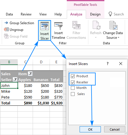
Two pivot table slicers are created immediately:

Tip. To filter your pivot table by various time periods, such as years, quarters, months, or days, you can add a timeline - a dynamic filter by date fields.
How to create a slicer for Excel table
In addition to pivot tables, the modern versions of Excel also let you insert a slicer for a regular Excel table. Here's how:
- Click anywhere in your table.
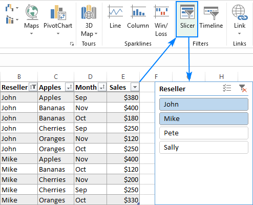
- On the Insert tab, in the Filters group, click Slicer.
- In the Insert Slicers dialog box, tick off the check boxes for one or more columns that you want to filter.
- Click OK.
That's it! A slicer is created and you can now filter your table data visually:
How to insert a slicer for pivot chart
To be able to filter a pivot chart with a slicer, you can actually make a slicer for your pivot table like explained above, and it will control both the pivot table and the pivot chart.
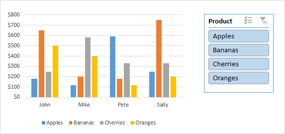
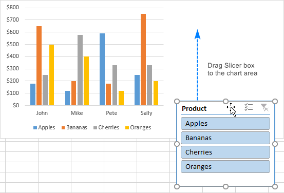
To integrate a slicer with your pivot chart more closely like shown in the screenshot above, carry out these steps:
- Click anywhere in your pivot chart.
- On the Analyze tab, in the Filter group, click Insert Slicer.
- Select the checkboxes for the slicer(s) you want to create, and click OK.
This will insert the already familiar slicer box in your worksheet:
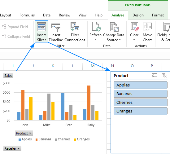
Once you have a slicer, you can use it to filter the pivot chart data straight away. Or, you may want to make a few improvements, for example, hide the filter buttons on the chart, which have become redundant since you are going to use the slicer for filtering.
Optionally, you can place the slicer box within the chart area. For this, make the chart area bigger and the plot arear smaller (simply by dragging the borders), and then drag the slicer box to the empty space:
Tips:
- If the slicer box gets hidden behind the chart, right-click the slicer, and select Bring to Front from the context menu.
- To enable automatic adjustment of the graph's size based on slicer selections, set the axis scale options to Auto.
How to use slicer in Excel
Excel slicers were designed as user-friendly filter buttons, so their use is simple and intuitive. The below sections will give you some hints on how to get started.
Slicer as a visual pivot table filter
Once a pivot table slicer is created, simply click on one of the buttons inside the slicer box to filter your data. The pivot table will update immediately to show only the data that matches your filter settings.
To remove a specific item from the filter, click the corresponding button in the slicer to unselect the item.

You can also use a slicer to filter data that are not shown in the pivot table. For example, we can insert the Product slicer, then hide the Product field, and the slicer will still filter our pivot table by product:

If multiple slicers are connected to the same pivot table and clicking a certain item inside one slicer makes some items in the other slicer greyed out, that means there is no data to display.
For example, after we select "John" in the Reseller slicer, "Cherries" in the Product slicer gets greyed out, indicating that John did not make a single "Cherries" sale:

Tip. To prevent pivot table column resizing when using a slicer, disable the Autofit column widths on update feature.
How to select multiple items in a slicer
There are 3 ways to select multiple items in an Excel slicer:
- Click the slicer buttons while holding the Ctrl key.
- Click the Multi-Select button (please see the screenshot below), and then click on the items one by one.
- Click anywhere inside the slicer box, and press Alt + S to toggle on the Multi-Select button. Select the items, and then press Alt + S again to toggle multi-selection off.

Move a slicer in Excel
To move a slicer to another position in a worksheet, put the mouse pointer over the slicer until the cursor changes to a four-headed arrow, and drag it to a new position.

Resize a slicer
As with most Excel objects, the easiest way to change the slicer's size is by dragging the edges of the box.
Or, select the slicer, go to the Slicer Tools Options tab, and set the desired height and width for your slicer:

Lock the slicer position in a worksheet
To fix the position of a slicer in a sheet, just do the following:
- Right click the slicer, and then click Size and Properties.
- On the Format Slicer pane, under Properties, select the Don't move or size with cells box.
This will keep your slicer from moving as you add or delete rows and columns, add or remove fields from the pivot table, or make other changes to the sheet.

Clear slicer filter
You can clear the current slicer settings in one of these ways:
- Click anywhere in the slicer box, and press the Alt + C shortcut.
- Click the Clear Filter button in the upper right corner.
This will remove the filter and select all items in the slicer:

Disconnect slicer from a pivot table
To disconnect a slicer from a given pivot table, here's what you do:
- Click anywhere in the pivot table from which you wish to disconnect a slicer.
- In Excel 2013 - 365, go to the Analyze tab > Filter group, and click Filter Connections. In Excel 2010, go to the Options tab, and click Insert Slicer > Slicer Connections.
- In the Filter Connections dialog box, clear the check box of the slicer you want to disconnect:

Please keep in mind that it won't delete the slicer box from your spreadsheet but only disconnect it from the pivot table. If you'd like to restore the connection later, open the Filter Connections dialog box again, and select the slicer. This technique might come in handy when the same slicer is connected to multiple pivot tables.
How to customize Excel slicer
Excel slicers are easily customizable - you can change their look and feel, colors, and settings. In this section, we will focus on how you can refine a slicer that Microsoft Excel creates by default.
Change slicer style
To change the default blue color of an Excel slicer, do the following:
- Click on the slicer for the Slicer Tools tab to appear on the ribbon.
- On the Slicer Tools Options tab, in the Slicer Styles group, click on the thumbnail you want to use. Done!
Tip. To see all available slicer styles, click the More button:

Create a custom slicer style in Excel
If you're not quite happy with any of the built-in Excel slicer styles, make your own one :) Here's how:
- On the Slicer Tools Options tab, in the Slicer Styles group, click the More button (please see the screenshot above).
- Click the New Slicer Style button at the bottom of the Slicer Styles gallery.
- Give a name to your new style.
- Select a slicer element, click the Format button, and choose the formatting options for that element. When finished, move on to the next element.
- Click OK, and your newly created style will appear in the Slicer Styles Gallery.

At first sight, certain slicer elements may sound confusing, but the below visual will hopefully give you some clues:
- "With Data" elements are slicer items associated with some data in the pivot table.
- "With no Data" elements are slicer items for which there is no data in the pivot table (e.g. the data was removed from the source table after a slicer was created).

Tips:
- If you are keen to create an awesome slicer design, but don't know where to start, choose the inbuilt style closest to your idea of a perfect slicer, right click it, and select Duplicate. Now, you can customize individual elements of that slicer style to your liking and save it under a different name.
- Since custom styles are saved at the workbook level, they are not available in new workbooks. To overcome this limitation, save the workbook with your custom slicer styles as an Excel Template (*.xltx file). When you create a new workbook based on that template, your custom slicer styles will be there.
Multiple columns in Excel slicer
When you have too many items in a slicer that do not fit within the box, arrange the items in multiple columns:
- With the slicer selected, go to the Slicer Tools Options tab > Buttons group.
- In the Columns box, set the number of columns to show inside the slicer box.
- Optionally, adjust the height and width of the slicer box and buttons as you see fit.
Now, you can select the slicer items without having to scroll up and down.

By using this approach, you can even make your slicer look like tabs behind your pivot table:

To achieve the "tabs" effect, the following customizations have been made:
- The slicer was set up in 4 columns.
- The slicer header was hidden (please see the instructions below).
- A custom style was created: the slicer border was set to none, the border of all items and the fill color of the "Selected item with data" was set to match the color of pivot table's header row. Please see How to create a custom slicer style for more details.
Change the slicer settings
One of the best things about Excel slicers is that they are fully customizable. You simply right-click the slicer, and click Slicer Settings… The Slicer Settings dialog box will show up (the screenshot below shows the default options):

Among other things, the following customizations might prove useful:
- Hide the slicer header by clearing the Display header box.
- Sort slicer items ascending or descending.
- Hide items with no data by unselecting the corresponding box.
- Hide items deleted from the data source by clearing the relevant check box. With this option unchecked, your slicer will stop showing old items that were removed from the data source.
How to connect slicer to multiple pivot tables
To build powerful cross-filtered reports in Excel, you may want to connect the same slicer to two or more pivot tables. Luckily, Microsoft Excel provides this feature too, and it does not require any rocket science :)
To link a slicer to multiple pivot tables, please follow these steps:
- Create two or more pivot tables, ideally, in the same sheet.
- Optionally, give meaningful names to your pivot tables so that you can easily identify each table by its name. To name a pivot table, go to Analyze tab and type a name in the PivotTable Name box in the top left corner.
- Create a slicer for any pivot table as usual.
- Right click on the slicer, and then click Report Connections (PivotTable Connections in Excel 2010).
Alternatively, select the slicer, go to the Slicer Tools Options tab > Slicer group, and click the Report Connections button.
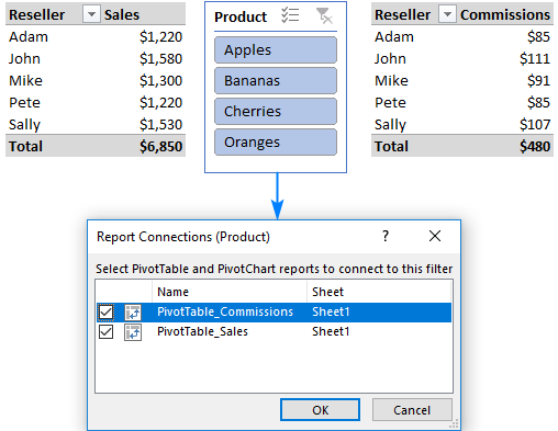
- In the Report Connections dialog box, select all the pivot tables you want to link to the slicer, and click OK.

From now on, you can filter all the connected pivot tables with a single click on a slicer button:
In the same manner, you can connect one slicer to multiple pivot charts:
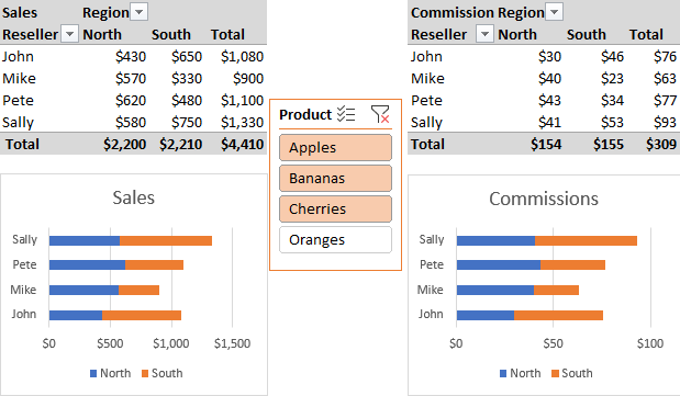
Note. One slicer can be connected only to those pivot tables and pivot charts that are based on the same data source.
How to unlock slicer in a protected worksheet
When sharing your worksheets with other users, you may want to lock your pivot tables from editing, but keep the slicers selectable. Here are the steps for this set up:
- To unlock more than one slicer at a time, hold the Ctrl key while selecting the slicers.
- Right click on any of the selected slicers and select Size and Properties from the context menu.
- On the Format Slicer pane, under Properties, uncheck the Locked box, and close the pane.

- On the Review tab, in the Protect group, click Protect Sheet.
- In the Protect Sheet dialog box, check the Use PivotTable & PivotChart option.

- Optionally, enter a password and click OK.
Please see How to protect and unprotect Excel worksheet for more information.
Now, you can share your worksheets even with Excel novices without worrying about the safety of your data - other users won't mangle the format and layout of your pivot tables, but will still be able to use your interactive reports with slicers.
How to remove a slicer in Excel
To permanently delete a slicer from your worksheet, do one of the following:
- Select the slicer and press the Delete key.
- Right-click the slicer, and then click Remove <Slicer Name>.
I hope this tutorial has shed some light on how to insert and use slicers in Excel. To gain more understanding, you are welcome to download our sample workbook with examples below. I thank you for reading and hope to see you on our blog next week!
Practice workbook for download
Excel Slicer examples (.xlsx file)
 by
by
23 comments
@Svetlana Cheusheva and Team.....thank you so much for all the beautiful content you publish via https://www.ablebits.com. It is so to the point, indepth, techincal and complete course - very much appreciated!!. I have to use Excel a lot nowadays in new job data, analysing massive data and I always check ABLEBITS.com ( for years now since i discovered site in 2014) when I get stuck, and quick reference uncomplicated explanations. Thank you. You are the best. A Quick question, do you do any online courses one can subscribe to and PAY....I feel so guilty all these years using your free resources - MAN has to earn and feed family in these hard times - I sure would register on one of your Excel courses to give back and help you publish more. I feel so guilty consuming free. Feel free inbox me. Thank you all the same and God bless. Anthony in England (currently stuck on massive cost analysis project for the NHS and needing to streamline my slow unresponsive excels and this has been useful)... lol lol.....THANK YOU!
Hi Anthony,
Thank you so much for your kind words! I am happy to hear my articles have been helpful. Ablebits does not run any training courses, but thank you for your willingness to subscribe. And good luck with your analysis project!
Good afternoon!
Is it possible to change the order in Slicer without using A to Z or Z to A sorting? Because I need another order in my Slicer
Hi!
Sorting in Slicer is the same as in Excel: from smallest to largest and vice versa. What sorting do you want?
I have an existing slicer and would like to color code the buttons based on a current value. Green for positive, Red for negative. How can I do this so when the value changes the button color automatically changes?
Hello!
Standard Excel conditional formatting can be applied only to cells. Conditional formatting of the slicer can be done using VBA.
Can a single slicer be used to filter multiple pivots from different data source table ?
Yes, it can. Please see How to connect a slicer to multiple pivot tables.
Hi Team,
Your tutorials are the best by far and by all standards.
Keep it up.
Hi Osorio,
Thank you so much for your kind words. We are delighted to hear this! :)
Good article on the incredibly useful slicer tool - wish I'd found this before I had to discover all that by trial and error!
Something useful that I don't think you mentioned. In Size and Properties - Position and Layout, you can Disable resizing and moving.
Even on a spreadsheet only used by myself it prevents accidentally shifting the Slicers.
Hi Tim,
Thank you for your feedback. These are very helpful options indeed! I mentioned them in the "Lock the slicer position in a worksheet" section.
Nice, indepth article. :-). You mentioned "Slicers perform great in touch screen environments." I completely agree, but what kind of touch screens? I have an iPad Pro and would LOVE the functionality of a slicer, either a Table Slicer OR Pivot Slicer. I can't get it to work and all the research I've found say it's not supported for iPads. Very depressing, unless you know the way how...?
Hi Kasper,
You are right, slicers do not work on iPads. On excel.uservoice.com, I've found a few requests to enable support for Pivot Tables and Slicers in iPad and Android, but Microsoft makes no promises for now though. I've added this caveat to the article, thank you for drawing my attention to this!
Thank you for letting me know about adding the caveat. I reread your article and when I noticed the IOS comment I was soo confused thinking how I could’ve missed that part. So I was happy when I saw your comment. Yes, it’s a shame they’re not compatible, but I’ve found a workaround. If you use the web based version of excel, Slicers WILL work on an Ipad. It’s a bit sluggish, so I’m hoping this feature will be added soon. Again, great article! I’ve recently starting working with Pivot tables and discovered the magic of slicers, so this article is a great reference.
In the graph, where did the North and South parameter came from. I didn't see it from the data.
Hi Emman,
As far as I understand you are asking about an image that shows a slicer connected to multiple pivot charts, right? That chart is created for a different data set, and I've updated the visual to show the original data. Sorry for the confusion!
Can you explain how to use a slicer selection in vlookup? I want to reference the slicer value across a difference data set to return a value.
I have used a similar feature to create dynamic Reports adjusting the slicer dates to "today' and "yesterday" (or "this week" and "prior" week"). What you need to do is create a new Table and add it to your data model, with at least two columns, one with field name: "Relative" with values: "today" and "yesterday", and a second column with field name: "Absolute" and enter the Excel functions =TODAY() and +TODAY()-1. You can then link the two data sets in your data model through fields "Date" (from your original source), and "Absolute" (from your newly created table) in your field lists. Once you have done that, create a slicer and select "Relative". You will get a dynamic slicer that will adjust automatically based on the date. This functionality should work just the same for a VLOOKUP(). All you need to do is to create your secondary table and enter your VLOOKUP() formula inside the Table.
very useful. Thanks. I was trying on the same line... but was not clear in my mind itself so I could not succeed. Now I will try. Thanks
Can we send a active slicer with graphs in the body of an outlook email. So that user can see the graph based on their filters
Hello!
To my best knowledge, it's not possible.
there is 3 column in a table and we have to marge it. we have also apply the slicer in this table. can we marge the 3 cell.