The tutorial shows how to use the VALUE function in Excel to convert text strings to numeric values.
Normally, Microsoft Excel recognizes numbers stored as text and converts them to the numerical format automatically. However, if the data is stored in a format that Excel cannot recognize, numeric values can be left as text strings making calculations impossible. In such situations, the VALUE function can be a quick remedy.
Excel VALUE function
The VALUE function in Excel is designed to convert text values to numbers. It can recognize numeric strings, dates and times.
The syntax of the VALUE function is very simple:
Where text is a text string enclosed in quotation marks or a reference to a cell containing the text to be changed to a number.
The VALUE function was introduced in Excel 2007 and is available in Excel 2010, Excel 2013, Excel 2016 and later versions.
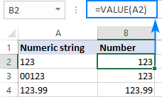
For example, to convert text in A2 to number, you use this formula:
=VALUE(A2)
In the screenshot below, please notice the original left-aligned strings in column A and the converted right-aligned numbers in column B:

How to use VALUE function in Excel - formula examples
As pointed our earlier, in most situations Excel converts text to numbers automatically when necessary. In some situations, however, you need to explicitly tell Excel to do so. The below examples show how this works in practice.
VALUE formula to convert text to number
You already know that the main purpose of the VALUE function in Excel is to change text strings to numeric values.
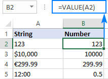
The following formulas give some ideas of what kind of strings can be turned into numbers:
| Formula | Result | Explanation |
| =VALUE("$10,000") | 10000 | Returns a numeric equivalent of the text string. |
| =VALUE("12:00") | 0.5 | Returns the decimal number corresponding to 12 PM (as it is stored internally in Excel. |
| =VALUE("5:30")+VALUE("00:30") | 0.25 | The decimal number corresponding to 6AM (5:30 + 00:30 = 6:00). |
The screenshot below shows a few more text-to-number conversions performed with the same VALUE formula:

Extract number from text string
Most Excel users know how to extract the required number of characters from the start, end or middle of a string - by using the LEFT, RIGHT and MID functions. When doing so, you have to remember that the output of all these functions is always text, even when you are extracting numbers. This may be irrelevant in one situation, but critical in another because other Excel functions treat the extracted characters as text, not numbers.
As you can see in the screenshot below, the SUM function is not able to add up the extracted values, though at first sight you may not notice anything wrong about them, maybe except for the left alignment typical for text:

In case you do need to use the extracted numbers in further calculations, wrap your formula into the VALUE function. For example:
To extract the first two characters from a string and return the result as a number:
=VALUE(LEFT(A2,2))
To extract two characters from the middle of a string beginning with the 10th char:
=VALUE(MID(A3,10,2))
To extract the last two characters from a string as numbers:
=VALUE(RIGHT(A4,2))
The above formulas not only pull the digits, but also perform the text to number conversion along the way. Now, the SUM function can calculate the extracted numbers without a hitch:

Of course, these simple examples are mostly for demonstration purposes and for explaining the concept. In real-life worksheets, you may need to extract a variable number of digits from any position in a string. The following tutorial shows how to do this: How to extract number from string in Excel.
VALUE function to convert text to dates and times
When used on dates/times text strings, the VALUE function returns a serial number representing the date or/and time in the internal Excel system (integer for date, decimal for time). For the result to appear as a date, apply the Date format to the formula cells (the same is true for times). For more information, please see Excel date format.
The screenshot below shows possible outputs:

Also, you can use the alternative ways to convert text to dates and times in Excel:
To convert date values formatted as text to normal Excel dates, use the DATEVALUE function or other ways explained in How to convert text to date in Excel.
To convert text strings to time, use the TIMEVALUE function as shown in Convert text to time in Excel.
Why Excel VALUE function returns #VALUE error
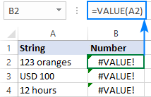
If a source string appears in a format not recognized by Excel, a VALUE formula returns #VALUE error. For example:

How do you fix this? By using more complex formulas described in How to extract number from string in Excel.
Hopefully this short tutorial has helped you to gain understanding about using the VALUE function in Excel. I thank you for reading and hope to see you on our blog next week!
Practice workbook for download
Excel VALUE formula - examples (.xlsx file)
 by
by
4 comments
Dear Sir,
I want to convert in numbers due to a gap in numbers I am unable to convert in numbers. please provide me with the formula.
State Sum of Outstanding
Goa -1,92,004
Gujarat 7,00,09,380
Himachal Pradesh -26,42,111
Jammu & Kashmir -32,63,118
Karnataka -18,01,730
Kerala -1,17,150
Madhya Pradesh -72,12,512
Maharashtra -23,45,478
Manipur -69,000
Meghalaya -68,550
Mizoram -68,750
Nagaland -85,55,860
Pudduchery -19,31,333
Punjab -78,42,539
Rajasthan 2,22,08,906
Sikkim -43,70,283
Tamil Nādu -1,00,24,496
Tripura -1,10,97,149
Uttar Pradesh -25,58,757
Uttarakhand 2,20,659
Grand Total -1,83,76,283
Hello!
Remove commas from your numbers with any of these methods. Then convert the text to a number using the VALUE function or use these guidelines.
I hope my advice will help you solve your task.
Hello,
Is it possible to give a letter a value in excel? I want to make "x" equal 1 so every time the letter "x" is placed in a column, the sum at the bottom of that column recognizes the "x" as a value of one and increases the sum at the bottom of the column. Is this possible or do I have to type the number 1 in each row in order to have a sum at the bottom?
Hi!
If "x" is in one column and values in another, it might be helpful to use the SUMIF function. If you describe the problem in more detail, perhaps I can give more precise recommendations.