In this tutorial, you will learn how to do a scatter plot in Excel to create a graphical representation of two correlated data sets.
When looking at two columns of quantitative data in your Excel spreadsheet, what do you see? Just two sets of numbers. Do you want to see how the two sets are related to each other? The scatter plot is the ideal graph choice for this.
Scatter plot in Excel
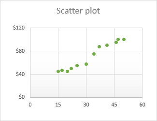
A scatter plot (also called an XY graph, or scatter diagram) is a two-dimensional chart that shows the relationship between two variables.
In a scatter graph, both horizontal and vertical axes are value axes that plot numeric data. Typically, the independent variable is on the x-axis, and the dependent variable on the y-axis. The chart displays values at the intersection of an x and y axis, combined into single data points.
The main purpose of a scatter plot is to show how strong the relationship, or correlation, between the two variables is. The tighter the data points fall along a straight line, the higher the correlation.
How to arrange data for a scatter chart
With a variety of inbuilt chart templates provided by Excel, creating a scatter diagram turns into a couple-of-clicks job. But first, you need to arrange your source data properly.
As already mentioned, a scatter graph displays two interrelated quantitative variables. So, you enter two sets of numeric data into two separate columns.
For ease of use, the independent variable should be in the left column as this column is going to be plotted on the x axis. The dependent variable (the one affected by the independent variable) should be in the right column, and it will be plotted on the y axis.
Tip. If your dependent column comes before the independent column and there is no way you can change this in a worksheet, you can the swap x and y axes directly on a chart.
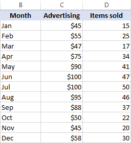
In our example, we are going to visualize the relationship between the advertising budget for a certain month (independent variable) and the number of items sold (dependent variable), so we arrange the data accordingly:
How to create a scatter plot in Excel
With the source data correctly organized, making a scatter plot in Excel takes these two quick steps:
- Select two columns with numeric data, including the column headers. In our case, it is the range C1:D13. Do not select any other columns to avoid confusing Excel.
- Go to the Inset tab > Chats group, click the Scatter chart icon, and select the desired template. To insert a classic scatter graph, click the first thumbnail:

The scatter diagram will be immediately inserted in your worksheet:
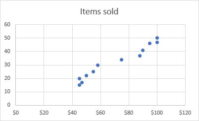
Basically, you may consider the work done. Or, you can customize some elements of your graph to make it look more beautiful and to convey the correlation between the two variables clearer.
Scatter chart types
Besides the classic scatter plot shown in the above example, a few more templates are available:
- Scatter with smooth lines and markers
- Scatter with smooth lines
- Scatter with straight lines and markers
- Scatter with straight lines
Scatter with lines is best to be used when you have few data points. For example, here's how you can represent the data for the first four months by using the scatter graph with smooth lines and markers:

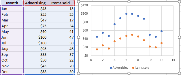
The Excel XY plot templates can also draw each variable separately, presenting the same relationships in a different way. For this, you should select 3 columns with data - the leftmost column with text values (labels), and the two columns with numbers.
In our example, the blue dots represent advertising cost, and orange dots represent the items sold:
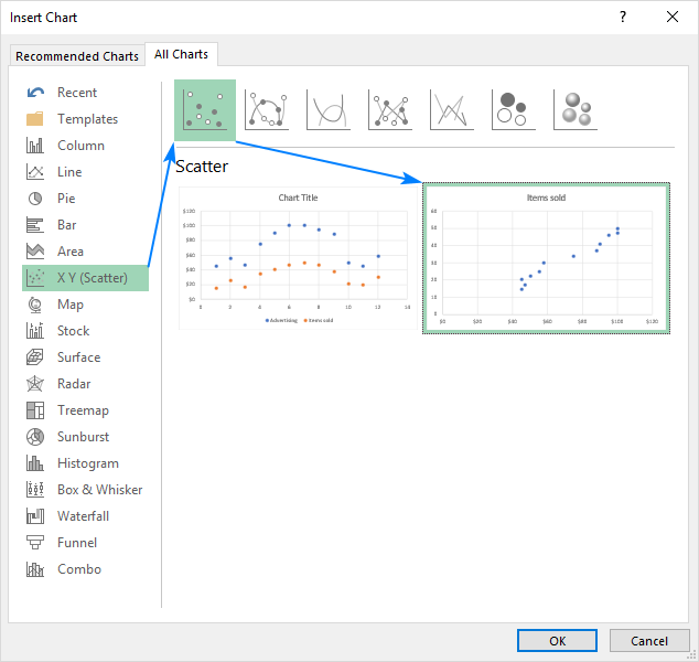
To view all available scatter types in one place, select your data, click the Scatter (X, Y) icon on the ribbon, and then click More Scatter Charts… This will open the Inset Chart dialog box with the XY (Scatter) type selected, and you switch between the different templates at the top to see which one provides the best graphic representation of your data:
3D scatter plot
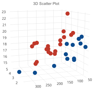
Unlike a classic XY scatter chart, a 3D scatter plot displays data points on three axes (x, y, and z) in order to show the relationship between three variables. Therefore, it is often called an XYZ plot.
Regrettably, there is no way to create a 3D scatter plot in Excel, even in the new version of Excel 2019. If you strongly need this chart type for your data analysis, consider using some third-party tool, like plot.ly. The screenshot below shows what kind of a 3D scatter graph this tool can draw:
Scatter graph and correlation
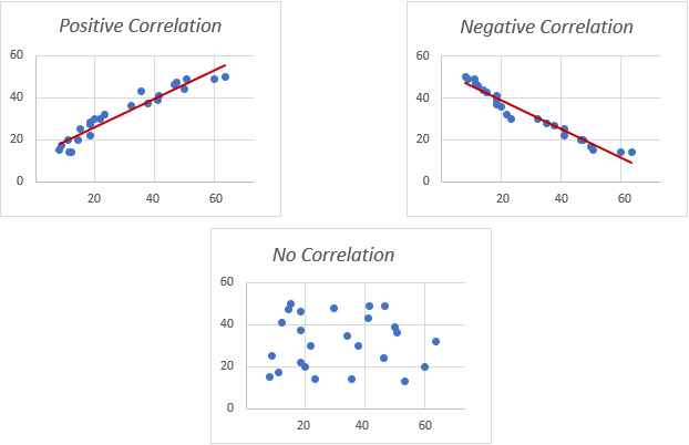
To interpret the scatter plot correctly, you need to understand how the variables can relate to each other. Overall, there exist three types of correlation:
Positive Correlation - as the x variable increases, so does the y variable. An example of a strong positive correlation is the amount of time the students spend studying and their grades.
Negative Correlation - as the x variable increase, the y variable decreases. Ditching classes and grades are negatively correlated - as the number of absences increases, the exam scores decrease.
No Correlation - there is no evident relationship between the two variables; the dots are scattered around the entire chart area. For example, students' height and grades appear to have no correlation as the former does not affect the latter in any way.
Customizing XY scatter plot in Excel
As with other chart types, nearly each element of a scatter graph in Excel is customizable. You can easily change the chart title, add axis titles, hide the gridlines, choose your own chart colors, and more.
Below we will focus on a few customizations specific to a scatter plot.
Adjust the axis scale (reduce white space)
In case your data points are clustered at the top, bottom, right, or left side of the graph, you may want to clean up the extra white space.
To reduce the space between the first data point and the vertical axis and/or between the last data point and the right edge of the graph, perform these steps:
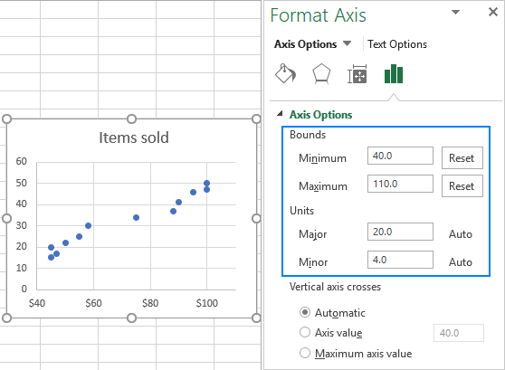
- Right-click the x axis, and click Format Axis…
- On the Format Axis pane, set the desired Minimum and Maximum bounds as appropriate.
- Additionally, you can change the Major units that control the spacing between the gridlines.
The below screenshot shows my settings:
To remove space between the data points and the top/bottom edges of the plot area, format the vertical y axis in a similar manner.
Add labels to scatter plot data points
When creating a scatter graph with a relatively small number of data points, you may wish to label the points by name to make your visual better understandable. Here's how you can do this:
- Select the plot and click the Chart Elements button.
- Tick off the Data Labels box, click the little black arrow next to it, and then click More Options…

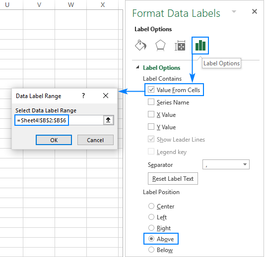
- On the Format Data Labels pane, switch to the Label Options tab (the last one), and configure your data labels in this way:
- Select the Value From Cells box, and then select the range from which you want to pull data labels (B2:B6 in our case).
- If you'd like to display only the names, clear the X Value and/or Y Value box to remove the numeric values from the labels.
- Specify the labels position, Above data points in our example.
That's it! All data points in our Excel scatter plot are now labeled by name:

Tip: How to fix overlapping labels
When two or more data points are very close to each other, their labels may overlap, as is the case with the Jan and Mar labels in our scatter diagram. To fix this, click on the labels, and then click on the overlapping one so that only that label gets selected. Point your mouse cursor to the selected label until the cursor changes to the four-sided arrow, and then drag the label to the desired position.
As the result, you will have a nice Excel scatter plot with perfectly legible labels:

Add a trendline and equation
To better visualize the relationship between the two variables, you can draw a trendline in your Excel scatter graph, also called a line of best fit.
To have it done, right click on any data point and choose Add Trendline… from the context menu.
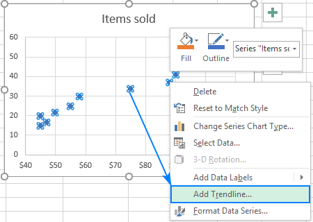
Excel will draw a line as close as possible to all data points so that there are as many points above the line as below.
Additionally, you can show the equation for the trendline that mathematically describes the relationship between the two variables. For this, check the Display Equation on Chart box on the Format Trendline pane that should appear in the right part of your Excel window immediately after you've added a trendline. The result of these manipulations will look similar to this:

What you see in the screenshot above is often called the linear regression graph, and you can find the detailed guidelines on how to create it here: How to make a linear regression graph in Excel.
How to switch X and Y axes in a scatter chart
As already mentioned, a scatter plot usually displays the independent variable on the horizonal axis and the dependent variable on the vertical axis. If your graph is plotted differently, the easiest fix is to swap the source columns in your worksheet, and then draw the chart anew.
If for some reason rearranging the columns is not possible, you can switch the X and Y data series directly on a chart. Here's how:
- Right-click any axis and click Select Data… in the context menu.
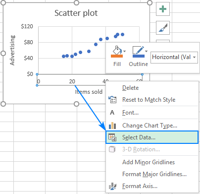
- In the Select Data Sourcedialog window, click the Edit button.

- Copy Series X valuesto the Series Y values box and vice versa.

Tip. To safely edit the contents of the Series boxes, put the mouse pointer in the box, and press F2.
- Click OK twice to close both windows.
As the result, your Excel scatter plot will undergo this transformation:

Tip. If you need to find a specific data point in a graph, this tutorial will teach you how to find, highlight and label a data point in a scatter plot.
That's how you create a scatter plot in Excel. In our next tutorial, we will continue with this topic and show how to quickly find and highlight a certain data point in a scatter graph. Please stay tuned!
 by
by
6 comments
This doesn't work - why the hell is Excel so counter-intuitive, you'd think selecting two columns of numeric data and clicking on scatter graph would make a simple scatter graph, wouldn't you? Not in the Microsoft world where the whole idea is that you need to be 'trained' to use Microsoft applications. Excel is, even more than it heretofore, an absolute piece of garbage.
You bet!
in "How to switch X and Y axes in a scatter chart" why do it? I can not understand this and I can not do this.
Hello!
In a a scatter plot, the independent variable is normally displayed on the horizonal axis (X) and the dependent variable on the vertical axis (Y). If, for whatever reason, your variables are plotted the other way round, you can swap the axes directly on the graph.
I do not have the plus button you have for your graph
Also, I have never said this so why am I getting a duplicate response?
Hi!
Just click anywhere on the chart for the plus button (Chart Elements button) to appear.
And sorry for the "duplicate response" message, our webmaster is working on it already.