In this tutorial, we will look at how you can join tables in Excel based on one or more common columns by using Power Query and Merge Tables Wizard.
Combining data from multiple tables is one of the most daunting tasks in Excel. If you decide to do it manually, you may spend hours only to find out that you've messed up important information. If you are an experienced Excel pro, then you can possibly rely on VLOOKUP and INDEX MATCH formulas. A macro, you believe, could do the job in no time, if only you knew how. The good news for all Excel users - Power Query or Merge Tables Wizard can be your time-saver. The choice is yours.
How to join tables with Excel Power Query
In simple terms, Power Query (also known as Get & Transform) is a tool to combine, clean and transform data from multiple sources into the format you need such as a table, pivot table or pivot chart.
Among other things, Power Query can join 2 tables into 1 or combine data from multiple tables by matching data in columns, which is the focus of this tutorial.
For the results to meet your expectations, please keep in mind the following things:
- Power Query is a built-in feature in Excel 2016 - Excel 365, but it can also be downloaded in Excel 2010 and Excel 2013 and used as an add-in. In your version, some windows may look different from the images in this tutorial that were captured in Excel 2016.
- For the tables to be combined correctly, they should have at least one common column (also referred to as a common id or key column or unique identifier). Also, the common columns should contain only unique values, with no repeats.
- The source tables can be located on the same sheet or in different worksheets.
- Unlike formulas, Power Query does not pull data from one table to another. It creates a new table that combines data from the original tables.
- The resulting table does not update automatically. You should explicitly tell Excel to do this. Please see how to refresh a merged table.
Source data
As an example, let's join 3 tables based on the common columns Order ID and Seller. Please note that our tables have different numbers of rows, and although table 1 has duplicates in the Seller column, table 3 contains only unique entries.
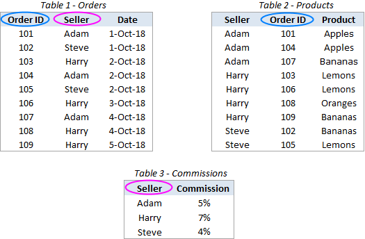
Our task is to map the data in table 1 with the relevant records from the other two tables, and combine all the data into a new table like this:

Before you start joining, I'd advise you to give some descriptive names to your tables, so it will be easier for you to recognize and manage them later. Also, although we say "tables", you do not actually need to create an Excel table. Your "tables" could be usual ranges or named ranges as in this example:
- Table 1 is named Orders
- Table 2 is named Products
- Table 3 is named Commissions
Create Power Query connections
Not to clutter your workbook with copies of your original tables, we are going to convert them into connections, do the merge within the Power Query Editor, and then load only the resulting table.
To save a table as a connection in Power Query, here's what you do:
- Select your first table (Orders) or any cell in that table.
- Go to the Data tab > Get & Transform group and click From Table/Range.

- In the Power Query Editor that opens, click on the Close & Load drop-down arrow (not the button itself!) and select the Close and Load To… option.

- In the Import Data dialog box, select the Only Create Connection option and click OK.

This will create a connection with the name of your table/range and display that connection in the Queries & Connections pane that appears on the right-hand side of your workbook.
- Repeat the above steps for all other tables you want to merge (two more tables, Products and Commissions, in our case).
When finished, you will see all the connections on the pane:

Merge two connections into one table
With the connections in place, let's see how you can join two tables into one:
- On the Data tab, in the Get & Transform Data group, click the Get Data button, choose Combine Queries in the drop-down list, and click Merge:
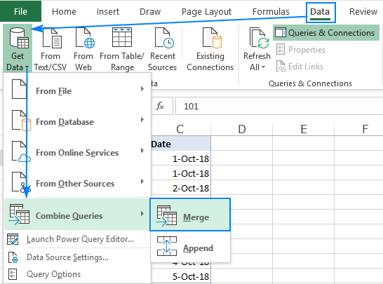
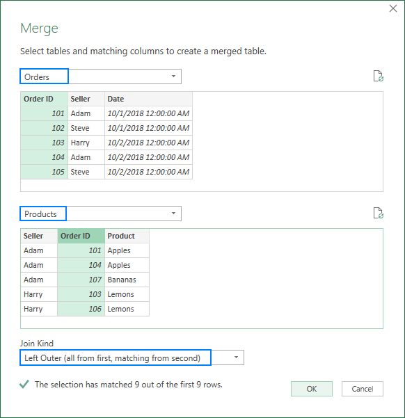
- In the Merge dialog box, do the following:
- Select your 1st table (Orders) from the first drop-down.
- Select your 2nd table (Products) from the second drop-down.
- In both previews, click on the matching column (Order ID) to select it. The selected column will get highlighted in green.
- In the Join Kind drop-down list, leave the default option: Left Outer (all from first, matching from second).
- Click OK.
Upon completion of the above steps, the Power Query Editor will show your first table (Orders) with one additional column named like your second table (Products) added to the end. This additional column does not have any values yet, just the word "Table" in all the cells. But don't feel discouraged, you did everything right, and we are going to fix that in a moment!
Select the columns to add from the second table
At this point, you have a table resembling the one in the screenshot below. To complete the merging process, perform the following steps within the Power Query Editor:
- In the added column (Products), click on the two-sided arrow in the header.

- In the box that opens, do this:
- Keep the Expand radio button selected.
- Unselect all columns, and then select only the column(s) you want to copy from the second table. In this example, we select only the Product column because our first table already has Seller and Order ID.
- Uncheck the Use original column name as prefix box (unless you want the column name to be prefixed with the table name from which this column is taken).
- Click OK.

As the result, you will get a new table that contains every record from your first table and the additional column(s) from the second table:

If you need to merge only two tables, you may consider the work almost done and go load the resulting table in Excel.
Merge more tables (optional)
In case you have three or more tables to join, there is some more work for you to do. I will outline the steps briefly here, because you have already done all this when joining the first two tables:
- Save the table you've got in the previous step (shown in the screenshot above) as a connection:
- In the Power Query Editor, click Close & Load drop-down arrow and select Close and Load To….
- In the Import Data dialog box, select Only Create Connection, and click OK.
This will add one more connection, named Merge1, to the Queries & Connections pane. You can rename this connection if you want (right-click and select Rename in the pop-up menu).

- Combine Merge1 with your third table (Commissions) by performing these steps (Data tab > Get Data > Combine Queries > Merge).
The screenshot below shows my settings:
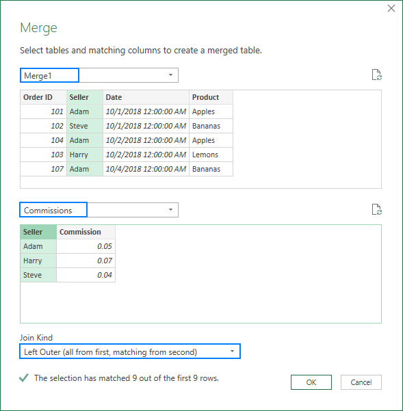
- Clicking OK in the Merge dialog box opens the Power Query Editor, where you select the columns to be added from table 3.
In this example, we add only the Commission column:

As the result, you get a merged table that consists of the first table, plus the additional columns copied from the other two tables.
Import the merged table to Excel
With the resulting table in the Power Query Editor, there is just one thing left for you to do - load it in your Excel workbook. And it is the easiest part!
- On the Home tab of the Power Query Editor, click the Close & Load drop-down arrow, and choose Close and Load To….
- In the Import Data dialog box, select Table and New Worksheet options.
- Click OK.

A new table combining the data from two or more sources appears in a new worksheet. Congratulations, you did it!
As a finishing touch, you may want to apply the right number format to some columns and maybe change the default table style to your favorite one. After these improvements, my combined table looks very nice:

Tip. If your tables contain numeric data (e.g. sales numbers or quantity) and you want a quick summary, you can load the resulting table as a PivotTable Report or create a pivot table in the usual way (Insert > PivotTable).
How to join tables based on multiple columns with Power Query
In the previous example, we were combining tables by matching data in one key column. But there is nothing that would prevent you from selecting two or more column pairs. Here's how:
In the Merge dialog box, hold the Ctrl key and click on the key columns one-by-one to select them. It is important that you click on the columns in the same order in both previews, so the matching columns have the same numbers. For example, Seller is key column 1 and Product is key column 2. Blank cells or rows that Power Query is unable to match show null:

After that, perform exactly the same steps as described above, and your tables will be merged by matching values in all the key columns.
How to update/refresh the merged table
The best thing about Power Query is that it is a one-time setup. When you make some changes to a source table, you don't have to repeat the whole process again. Simply, click the Refresh button on the Queries & Connections pane, and the merged table will update at once:

If the pane has disappeared from your Excel, click the Queries & Connections button on the Data tab to get it back.
Alternatively, you can click the Refresh all button on the Data tab tab or the Refresh button on the Query (this tab activates once you select any cell within a merged table).

Merge Tables Wizard - quick way to join 2 tables in Excel
Now that you are familiar with the inbuilt tool, let me show you our approach to merging tables in Excel.
In this example, we will be combining the same tables that we joined with Power Query a moment ago. I have just added a few more rows to the second table to show you more capabilities of our add-in:

With the Merge Tables Wizard installed in your Excel, here's what you need to do:
- Select the first table or any cell in it and click the Merge Two Tables button on the Ablebits Data tab:

- Take a quick look at the selected range to make sure the add-in got it right and click Next.

- Select the second table and click Next. Please note that our second table contains 26 rows compared to only 10 rows in the first table:

- Choose one or several matching columns and click Next. Since we are joining two tables by one common column, Order ID, we select only that column:
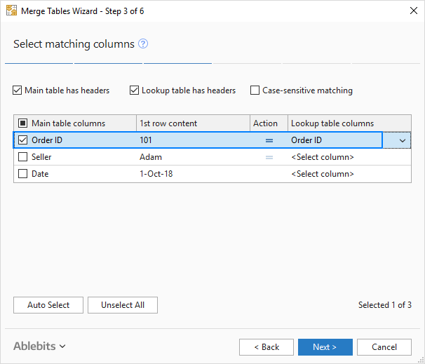
Please notice the Case-sensitive matching box at the top. Select it if you want to treat uppercase and lowercase text in the key columns as different characters. For this example, we don't need that, so we leave the box unselected. - Select the columns to update in the first table. This step is optional, and if you don't want any updates, you can click Next without selecting anything here.
We select the Seller column because we have more rows in the second table and we want the new seller names to appear in the existing Seller column:

- Choose the column(s) to be added to the first table, Product in our case, and click Next:

- This step is very important because it determines how your tables will be merged.
In this example, we go with the default options shown in the screenshot below. But I'd like to draw your attention to the following 2 boxes that can prevent overwriting your existing data in case you've chosen to update some columns:- Empty cells only
- Only if cells in the lookup table contain data
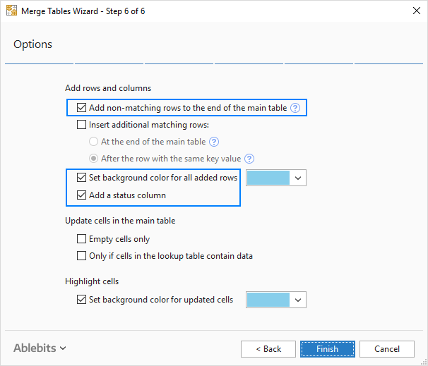
Make your choices, click Finish, allow the wizard a few seconds for processing, and examine the results.
With the default options, the wizard highlights the newly added rows and adds the Status column. If you don't want any of that, clear the corresponding boxes in the last step.

To join three and more tables, simply repeat the above steps. Just remember to select the result of a previous merge as your main table.
Unlike Power Query, the Merge Tables Wizard does not keep a connection between the resulting and source tables. In some situations, this may be a disadvantage. On the plus side, no matter what you do with the source table - edit, move or even delete - the merged table remains intact.
This example has shown just one scenario that our wizard can handle, but there is much more to it! If you are curious to know other use cases, please check out these examples.
Also, you can download a a trial version of Ultimate Suite for Excel that includes Merge Tables Wizard as well as 70+ other useful tools.
In case you are looking to join tables in some other way, you may find the following resources useful.
Other ways to combine data in Excel
- Merge tables by column headers - join two or more tables based on column names. You can choose to combine all the columns or only the ones you select.
- Combine multiple worksheets into one - copy multiple sheets into one summary worksheet. Of course, it's not manual copy/pasting! You only indicate which worksheets to merge, and our Copy Sheets tool does the rest.
- Compare two Excel files - how to compare two tables (worksheets) for differences and merge them into a single sheet.
 by
by
15 comments
I need to download a new source table every month. How do I ensure that the merged table remain linked? Do I need to make sure that the document is named the same and in the same directory?
Hi! If you are using Power Query to create a table join, make sure that the source table has the same name and is in the same directory. Unlike Power Query, the Merge Tables Wizard doesn’t store the relationship between the resulting and source tables.
Is it possible to do this using tables from different files? I need to do exactly what is in this article but the tables are in different files with different structures e.g. file 1 has name, email and town and file 2 has name, orders and returns. I want to merge these two using 'name' as that is the same and I want to be able to automate this every time there is a new version of files 1 and 2. Thanks
Hi! You can merge tables from different files by key column using the Merge Tables Wizard. It is available as a part of our Ultimate Suite for Excel that you can install in a trial mode and check how it works for free.
I have 30 sheets representing data from 30 different venues, the data set is exactly the same in each table/venue. In order to create a pivot table and graph to represent the results and KPIs between each venue, I need to merge the sheets into one long table so that all the results and venue names can be filtered displayed and compared against each other. The tables are all reading from external data sheets and populating into one master spreadsheet.
I could do this with formulas and index matching, but that is labor intensive, is there a simple way to basically append each table to each other?
You dont need to combine the data using these steps you just need to save all the data files in the same folder, then "get data" --->"from folder" and it will combine all the data into one which can then be formatted and imported into a pivot table which can then be processed as you describe.
Note this will only work if all the data files are laid out the same way and have the same data in each column i.e. venue name in column one date column 2, sales column 3 etc
i followed the steps to join/ merge but it appears that the data, from 10K rows are now 40K rows. means there are duplicates. is there a way to just map, instead of merge/ join?
Hi!
You can remove duplicates using the Duplicate Remover tool. It is available as a part of our Ultimate Suite for Excel. You can read more about removing duplicates in this article: How to remove duplicates in Excel (duplicate rows, values and partial matches).
Good morning:
In excel I have two long lists of names with some overlap. the first list is of people who have one talent, people on the second list have different talent. I want to find out who has both talents, who talent A but not talent B and viceversa.
How do advise that I proceed?
thanks
Hello!
I recommend reading this guide: How to compare two Excel files for differences.
Compare Sheets tool will help you quickly find and highlight differences between two Excel spreadsheets or lists.
how do i combine tables with information of sales of different days into one table spread on one excel sheet
Hello!
We have a tool that can solve your task in a couple of clicks: Ablebits Data - Merge Tables.
This tool is available as a part of our Ultimate Suite for Excel that you can install in a trial mode and use for free: https://www.ablebits.com/files/get.php?addin=xl-suite&f=free-trial
Using Excel 2016... any idea why the 'Join Kind' dropdown would be missing from my 'Merge' tab? The ONLY option I have at bottom of this tab is a check box to "only include matching rows".
Hello!
A drop-down list is a control that allows you to enter data in cells of your table. The Merge operation can be performed only with data from an Excel table, controls are not transferred to another table during the merge.