The tutorial shows how to do time series forecasting in Excel with the built-in Forecast Sheet feature and your own formulas.
In statistics, there exist many different forecasting techniques and some of these techniques are already implemented in Excel. This tutorial will teach you how to forecast in Excel based on historical data and may help you save money on specialized forecasting software :)
Forecast in Excel
Forecasting is a special technique of making predictions for the future by using historical data as inputs and analyzing trends.
This method is commonly used to make educated guesses on cash flows, plan budgets, anticipate future expenses or sales, and so on. However, forecasting doesn't tell the future definitively, it only shows probabilities. So, you should always double check the results before making a decision.
Microsoft Excel offers a few different forecasting tools including built-in features, functions, and graphs. Depending in your needs, you can choose one of the following methods:
- Exponential smoothing forecast - time series forecasting based on historical data with seasonal or other cycles.
- Linear forecast - predicting future values using linear regression.
How to forecast in Excel using exponential smoothing
Exponential smoothing forecasting in Excel is based on the AAA version (additive error, additive trend and additive seasonality) of the Exponential Triple Smoothing (ETS) algorithm, which smoothes out minor deviations in past data trends by detecting seasonality patterns and confidence intervals.
This forecasting method is best suited for non-linear data models with seasonal or other recurring patterns. It is available in Excel 2016, Excel 2019 and Excel for Office 365.
You can do such a forecast with your own formulas or have Excel create a forecast sheet for you automatically.
Create an exponential forecast sheet automatically
The Forecast Sheet feature introduced in Excel 2016 makes time series forecasting super-easy. Basically, you only need to appropriately organize the source data, and Excel will do the rest.
Arranging data
In your Excel worksheet, enter two data series into adjacent columns:
- Time series - date or time entries that are observed sequentially at a regular interval like hourly, daily, monthly, yearly, etc.
- Data values series - corresponding numeric values that will be predicted for future dates.
It is important that your time series have equal intervals between the data points. For example, you can supply weekly intervals with values on every Monday, monthly intervals with values on the 1st day of every month, etc.
In theory, your time series can miss up to 30% of data points or have several entries with the same date or time, and Excel will still do the forecast correctly. However, it is recommended to summarize your data to get more accurate predictions.
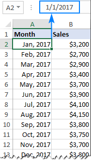
In this example, we will try to forecast sales for the next few years based on the following historical data. Please pay attention that column A contains dates (the 1st of every month) in a custom format that displays only the month and year. However, these are fully-functional dates, not text values.
Creating a forecast sheet
With the two data series in place, carry out the following steps to build a forecasting model:
- Select both data series. In most cases, it is sufficient to select just one cell in any of your series, and Excel picks up the rest of the data automatically.
- Go to the Data tab > Forecast group and click the Forecast Sheet button.

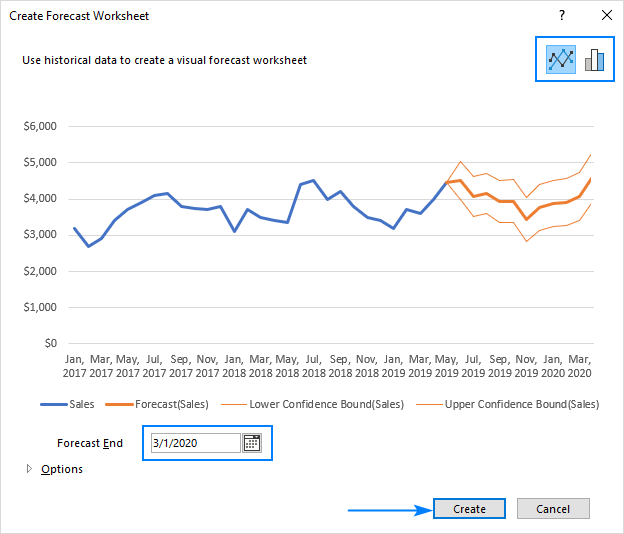
- The Create Forecast Worksheet window shows a forecast preview and asks you to choose:
- Graph type: line (default) or column chart
- End date for forecasting
- When done, click the Create button.
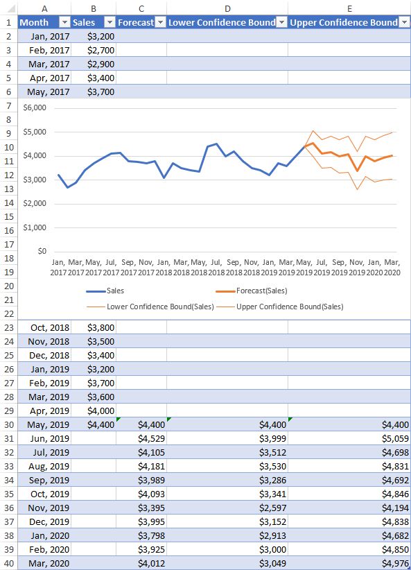
Excel immediately creates a new sheet containing a table with your original and predicted values as well as a chart that visually represents this data.
Here's how our Excel sales forecast looks like:
To find out how the predictions are calculated, click on one of the future values in your forecast worksheet and investigate the formula. Or check out Exponential smoothing forecast formulas for a quick overview.
Customizing Excel forecast
If you'd like to change any of the default options of your forecast, click Options in the lower-left part of the Create Forecast Worksheet window and configure the following settings the way you need:
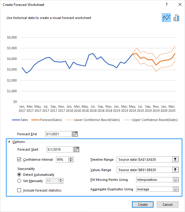
Forecast Start - the start date for forecasting. You can either select a date from the date picker or type it directly in the box.
- If your data is seasonal, it is recommended to start a forecast before the last historical point.
- To see how well the predictions match the known values, pick a date before the end of the historical data. In this case, only data prior to the start date will be used for forecasting (this back-testing method is also known as hindcasting).
Confidence Interval - a range in which the predictions are expected to fall. On the line chart, it is represented by the two finer lines on each side of the forecast line; on the column chart - by the error bar values.
Confidence interval can help you understand the forecast accuracy. A smaller interval indicates more confidence for a specific point. The default level is 95%, meaning that 95% of future points are expected to fall within the range.
You can check and uncheck the Confidence Interval box to show or hide it. And you can change the default value by using the up or down arrows.
Seasonality - the length of the seasonal pattern in which regular and predictable data fluctuations occur. For example, in a yearly pattern where each data point represents a month, the seasonality is 12.
Excel identifies the seasonal cycle automatically but also allows you to set it manually. When Excel is unable to detect seasonality (usually, with less than 2 cycles of historical data), the predictions revert to a linear trend.
Include Forecast Statistics - additional statistical information on the forecast. Check this box if you want Excel to generate a table of additional statistics such as smoothing constants (Alpha, Beta, Gamma) and error metrics (MASE, SMAPE, MAE, RMSE). All these values are calculated by using the FORECASE.ETS.STAT function.
Timeline Range - the range used for your timeline series. By default, it includes all dates in your source table, but you can change it here.
Values Range - the range used for your value series. It should match the Timeline Range.
Fill Missing Points Using - controls how missing points are handled. By default, Excel uses the Interpolation approach where the missing points are filled based on the weighted average of neighboring points. Alternatively, you can select Zeros to treat the missing points as zero values.
Duplicate Aggregates Using - determines how multiple values with the same timestamp are calculated. The default option is the average, but you can pick any other calculation method from the list, e.g. Median, Max or Min.
Exponential smoothing forecast formulas
A forecast sheet created by Excel contains two columns with your original data (timeline series and the corresponding data series) and three calculated columns (forecast values and two confidence bounds).
Naturally, nothing prevents you from building a similar forecasting model yourself by using the following formulas.
Forecasted values (FORECAST.ETS function)
The future values are calculated with the FORECAST.ETS function, which has the following syntax:
For the detailed explanation of each argument, please check out Using FORECAST.ETS function in Excel.
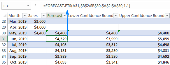
For our sample forecast sheet, Excel has created this formula:
=FORECAST.ETS(A31, $B$2:$B$30, $A$2:$A$30, 1, 1)
Where:
- A31 is the target date
- $B$2:$B$30 is the data values range
- $A$2:$A$30 is the time series range
- 1 in the 4th argument (seasonality) - tells Excel to detect seasonality automatically.
- 1 in the 5th argument (data completion) - tells Excel to complete missing points as the average of the neighboring points.
- The 6th argument (aggregation) is omitted, which means that multiple values with the same time stamp are to be aggregated using AVERAGE.
Confidence interval (FORECAST.ETS.CONFINT function)
To return a confidence interval for the forecast value at a specified date, the FORECAST.ETS.CONFINT function is used.
For our sample data set, the confidence interval can be calculated with this formula:
=FORECAST.ETS.CONFINT(A31, $B$2:$B$30, $A$2:$A$30, 0.95, 1, 1)
Where:
- A31 is the target date
- $B$2:$B$30 is the data values range
- $A$2:$A$30 is the time series range
- 0.95 - the confidence level is equal to 95%.
- 1 in the 5th argument (seasonality) - automatic detection of seasonality.
- 1 in the 6th argument (data completion) - missing points are completed based on the average of the neighboring points.
- 7th argument omitted (aggregation) - aggregate multiple data values with the same time stamp by using the AVERAGE function.
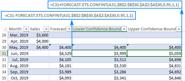
In the automatically created Forecast Sheet, Excel does not output the confidence interval value. Instead, it uses the FORECAST.ETS.CONFINT function in combination with the forecast value to calculate the Confidence Bounds, provided the Confidence Interval box is checked in the Options section.
To get the lower bound, you subtract the confidence interval from the forecasted value:
=C31 - FORECAST.ETS.CONFINT(A31, $B$2:$B$30, $A$2:$A$30, 0.95, 1, 1)
To get the upper bound, you add the confidence interval to the forecasted value:
=C31 + FORECAST.ETS.CONFINT(A31, $B$2:$B$30, $A$2:$A$30, 0.95, 1, 1)
Where C31 is the forecasted value returned by FORECAST.ETS.
How to forecast using linear regression in Excel
For data without seasonality or other cycles, you can predict future values by using linear regression. This method is also suited for small and simple data sets that do not have enough historical data to detect seasonality.
Microsoft Excel does not provide a built-in feature to do linear forecasting automatically, but it does have a special function for this, more precisely, two functions: FORECAST and FORECAST.LINEAR.
Both functions have the same purpose, syntax and return the same results. The difference is only in Excel versions:
- In Excel 2016 and Excel 2019, both functions are available, but it is recommended to use newer FORECAST.LINEAR.
- In Excel 2013, 2010 and 2007, only the FORECAST function is available.
The detailed explanation of the functions' syntax can be found in this tutorial: How to use FORECAST function in Excel. For now, let's focus on a liner forecast example.
Linear forecast formulas
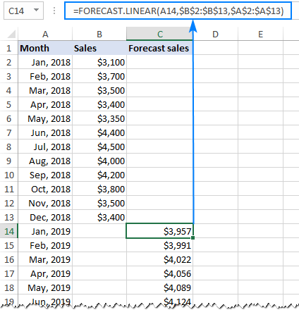
Suppose you have the sales data for the previous year and want to predict this year sales. With just one cycle of historical data, Excel cannot identify a seasonality pattern, therefore exponential smoothing is not an option. Well, let's do linear forecast with one of these formulas:
In Excel 2016 and 2019:
=FORECAST.LINEAR(A14, $B$2:$B$13, $A$2:$A$13)
In Excel 2013 and earlier versions:
=FORECAST(A14, $B$2:$B$13, $A$2:$A$13)
Where:
- A14 is the target date
- $B$2:$B$13 is the data values range
- $A$2:$A$13 is the time series range
Please pay attention that we lock both ranges with absolute cell references to prevent them from changing when we copy the formula down the column.
So, you enter one of the above formulas in any empty cell in row 14, drag it down to as many cells as needed, and have this result:
Linear regression forecasting graph
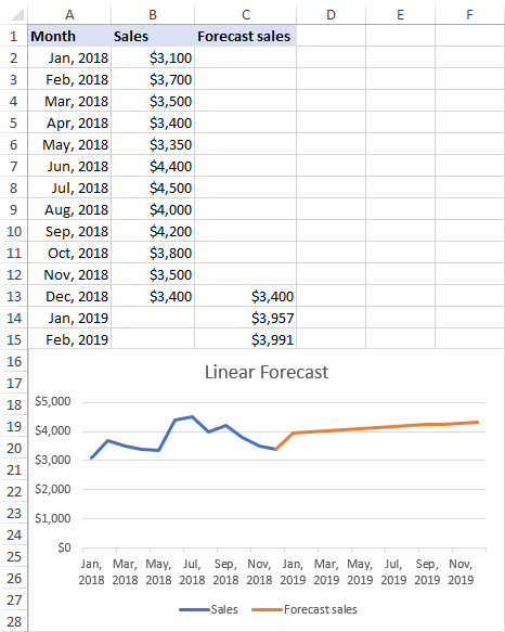
To better understand the future strategies, you can visually represent the predicted values in a line chart.
To draw a linear forecast graph like shown in the screenshot below, here's what you need to do:
- Copy the last historical data value to the Forecast In this example, we copy the value from B13 to C13. This will help us achieve the effect of a continuous uninterrupted line.
- Select 3 columns of data: time series, historical data values and forecasted values.
- On the Insert tab, in the Charts group, click the Insert Line or Area Chart icon and choose the first chart type (2-D Line).
Done!
That's how to do forecasting in Excel. To have a closer look at the examples discussed in this tutorial, you are welcome to download our Excel Forecast Sample Workbook.
I thank you for reading and hope to see you on our blog next week!
 by
by
5 comments
Hi
When forecasting on a worksheet and also using the formula, my results go into minus numbers.
The dataset used is consumption data and therefore cannot go into negative numbers.
Is there a way to set the forecast to only include numbers above 0?
I have this data -
1, Total Applications submitted in last 3 months
What I need to find "Applications that will be going to submit in upcoming next month'?
Please help me regarding this problem I am new in the "Data analysis".
Thanks you so much.
1. The following table shows sales of a shoe company during years 2020 and 2021.
Forecast the next four points, i.e., Spring, Summer, Fall, and Winter of 2022.
Date # of shoes sold
Spring 2020 9000 D1
Summer 2020 12000 D2
Fall 2020 8000 D3
Winter 2020 4000 D4
Spring 2021 8500 D5
Summer 2021 13000 D6
Fall 2021 7500 D7
Winter 2021 3300 D8
2. Use the same table in the question one and this time use the moving average
method to forecast F5, F6, F7, F8
Hi!
Please re-check the article above since it covers your task. You can learn more about moving average in Excel in this article on our blog.
How can I make smmorhing linear trend for quarterly data if I only have annual data?