You may think percentage calculations are useful only if you use them for work. But in reality, they help you in everyday life. Do you know how to tip properly? Is this discount a real deal? How much will you pay with this interest rate? Come find the answers to these and other similar questions in this article.
What is percentage
As you most likely already know, percent (or per cent) means one-hundredth part. It is marked by a special sign: %, and represents a part of the whole.
For example, your and your 4 friends are getting a birthday gift for another friend. It costs $250 and you're chipping in together. What percent of the total you're investing in the present?
This is how you usually calculate percents:
Let's see: you're giving away $50. 50/250*100 – and you get 20% of the gift cost.
However, Google Sheets makes the task simpler by calculating some parts for you. Below I'll show you those basic formulas that will help you get different results depending on your task, whether calculating percentage change, percentage of the total, etc.
How to calculate percentage in Google Sheets
This is how Google spreadsheet calculates percentage:
Unlike the previous formula, this one doesn't multiply anything by 100. And there's a good reason for that. Simply set the format of cells to percent and Google Sheets will do the rest.
So how will this work on your data? Imagine you keep track of ordered and delivered fruits (columns B and C respectively). To calculate the percentage of what's been received, do the following:
- Enter the below formula to D2:
=C2/B2 - Copy it down your table.
-
Go to Format > Number > Percent in Google Sheets menu to apply the percentage view.
Note. You'll need to go over these steps to create any percentage formula in Google Sheets.
Tip. You can decrease and increase decimal places if necessary using the options from the Google toolbar:

Here's how the result looks on real data:
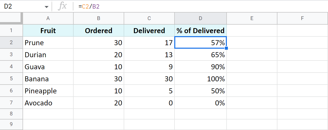
I removed all decimal places making the formula show the result as a rounded percent.
Percentage of a total in a Google spreadsheet
Here are a few more examples of calculating percentage of a total. Though the previous shows the same, it works great for that example but may not be enough for other data set. Let's see what else Google Sheets offers.
A common table with a total at its end
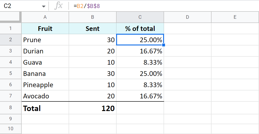
I believe this is the most common case: you have a table with values in column B. Their total resides at the very end of the data: B8. To find the percentage of the total for each fruit, use the same basic formula as before but with a slight difference – an absolute reference to the cell with the total sum.
This type of reference (absolute, with a dollar sign) doesn't change when you copy the formula to other cells. Thus, each new record will be calculated based on the sum in $B$8:
=B2/$B$8
I also formatted the results as percent and left 2 decimals to display:
One item takes a few rows – all rows are part of the total
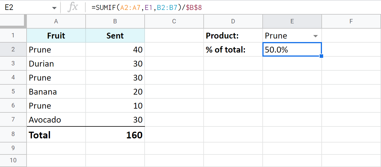
Now, suppose a fruit appears more than once in your table. What part of the total is composed of all deliveries of that fruit? The SUMIF function will help answer that:
It will sum only numbers belonging to the fruit of interest and divide the result by the total.
See for yourself: column A contains fruits, column B – orders for each fruit, B8 – the total of all orders. E1 has a drop-down list with all possible fruits where I chose to check the total for Prune. Here's the formula for this case:
=SUMIF(A2:A7,E1,B2:B7)/$B$8
Tip. Having a drop-down with fruits is completely up to you. Instead, you can put the necessary name right to the formula:
=SUMIF(A2:A7,"Prune",B2:B7)/$B$8
Tip. You can also check a part of the total made by different fruits. Just add up a few SUMIF functions and divide their result by the total:
=(SUMIF(A2:A7,"prune",B2:B7)+SUMIF(A2:A7,"durian",B2:B7))/$B$8
Percentage increase and decrease formulas
There's a standard formula you can use to calculate percent change in Google Sheets:
=(B-A)/A
The trick is to figure out which of your values belong to A and to B.
Let's assume you had $50 yesterday. You have saved $20 more and today you have $70. This is 40% more (increase). If, on the contrary, you've spent $20 and have only $30 left, this is 40% less (decrease). This deciphers the formula above and makes it clear which values should be used as A or B:
Let's see how this works in Google Sheets now, shall we?
Work out percent change from column to column
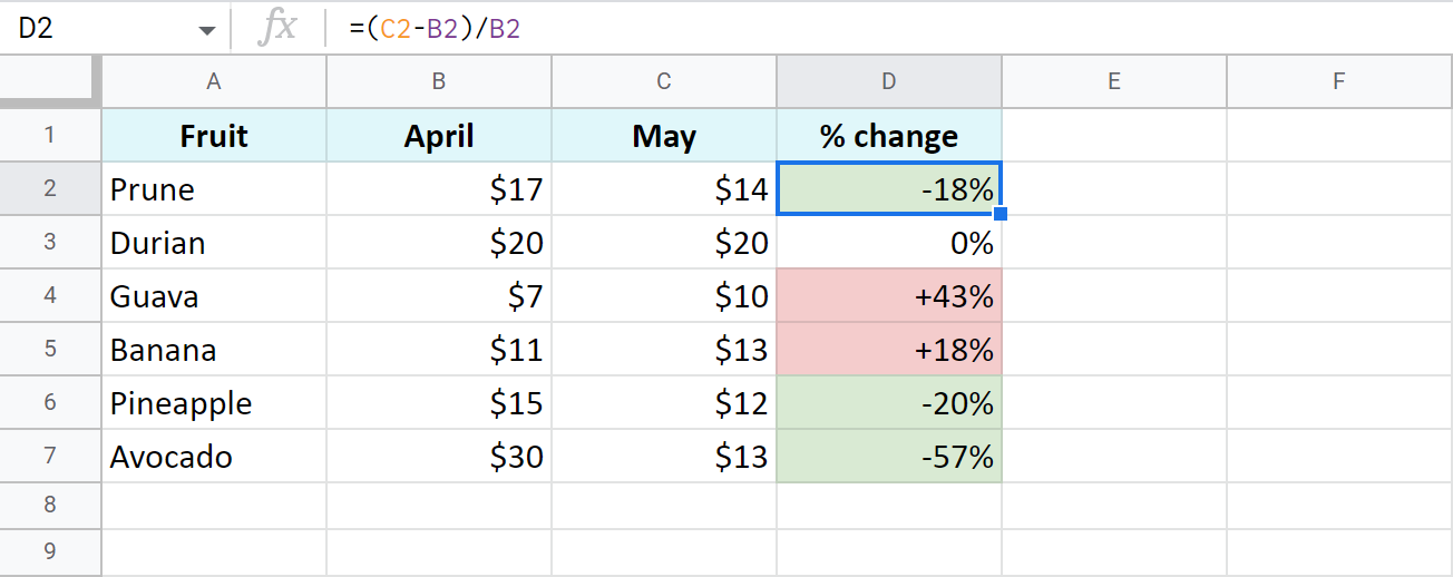
I have a list of fruits (column A) and I want to check how prices have shifted in this month (column C) compared to the previous one (columns B). Here's the percent change formula I use in Google Sheets:
=(C2-B2)/B2
Tip. Don't forget to apply the percent format and adjust the number of decimal places.
I also used conditional formatting to highlight cells with percent increase with red and percent decrease with green:
Percent change from row to row
This time, I'm tracking total sales (column B) over each month (column A). To make sure my formula works correctly, I should start entering it from the second row of my table – C3:
=(B3-B2)/B2
Copy the formula over all rows with data, apply the percent format, decide on the number of decimals, and voila:
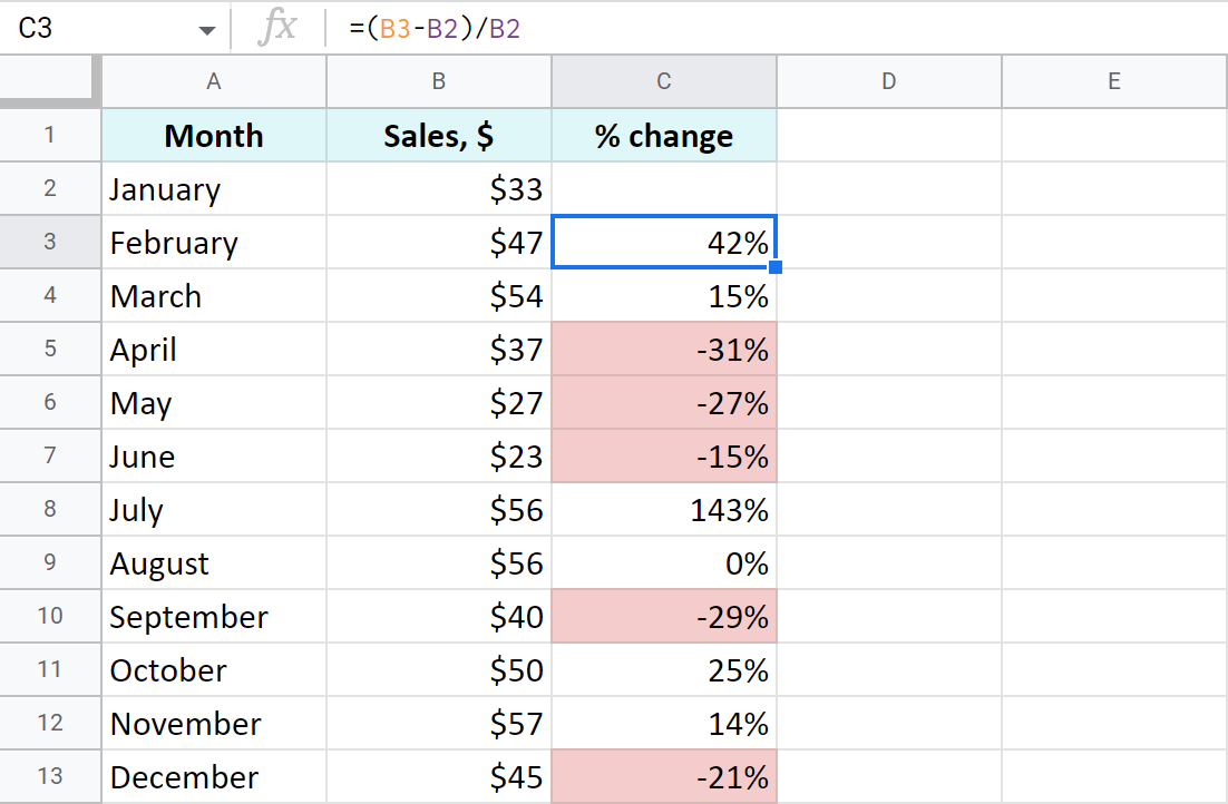
Here I also coloured percentage decrease with red.
Percent change compared to one cell
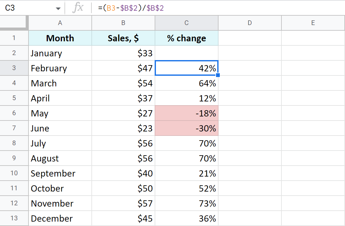
If you take the same sales list and decide to calculate percentage change based on January only, you will have to always refer to the same cell – B2. For that, make the reference to this cell absolute instead of relative so it doesn't change after copying the formula to other cells:
=(B3-$B$2)/$B$2
Amount and total by percentage in Google spreadsheets
Now that you've learned how to operate percentages, I hope getting total and the amount will be a child's play.
Find amount when having total and percentage
Let's imagine you've spent $450 shopping abroad and you'd like to have the taxes returned – 20%. So how much exactly should you expect to receive back? How much is 20% of $450? Here's how you should count:
If you put the total to A2 and the percent to B2, the formula for you is:
=A2*B2

Find total if you know amount and percentage
Another example: you've found an ad where a used scooter is being sold for $1,500. The price already includes a pleasant 40% discount. But how much would you need to pay for a new scooter like that? The below formula will do the trick:
As the discount is 40%, it means you are to pay 60% (100% – 40%). With these numbers at hand, you can work out the original price (total):
=A2/C2

Tip. As Google Sheets stores 60% as one hundredth – 0.6, you can get the same result with these two formulas as well:
=A2/0.6
=A2/60%
Increase and decrease numbers by percentage
The following examples represent the formulas you may need a bit more often than other ones.
Increase a number in a cell by percent
A general formula to calculate the raise by some percent is as follows:
If you have some amount in A2 and you need to increase it by 10% in B2, here's your formula:
=A2*(1+B2)

Decrease a number in a cell by percent
To make the opposite and decrease the number by a percent, use the same formula as above but replace the plus sign with a minus:
=A2*(1-B2)

Increase and decrease a whole column by percent
Now assume you have lots of records written in a column. You need to raise each of them by a percentage in that same column.
There's a quick way (6 steps to be exact) to do that with our Power Tools add-on for Google Sheets.
- Select all values you'd like to raise first and apply the automatic format: Format > Number > Automatic:
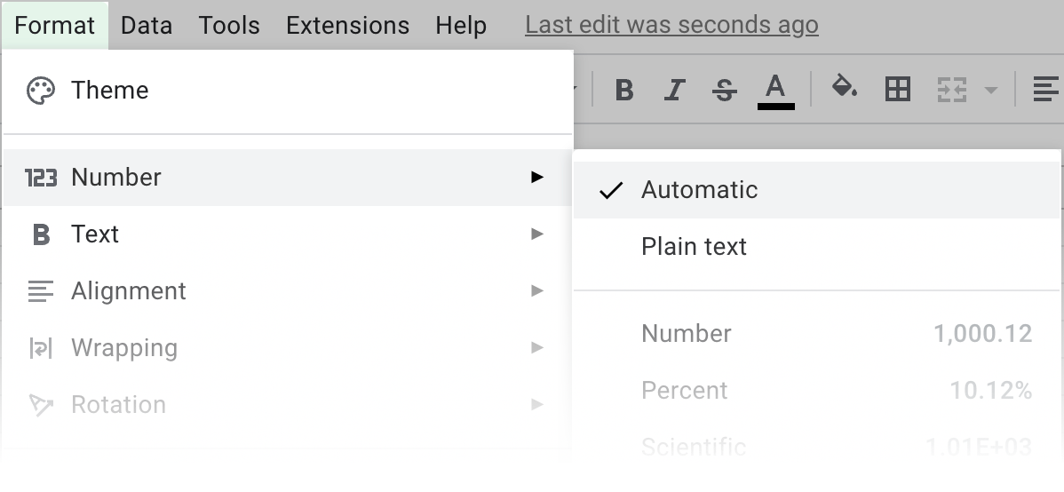
Note. This is required to avoid problems with formats on the next steps.
- Keep the values selected and run the Text tool from Extensions > Power Tools > Tools > Text:
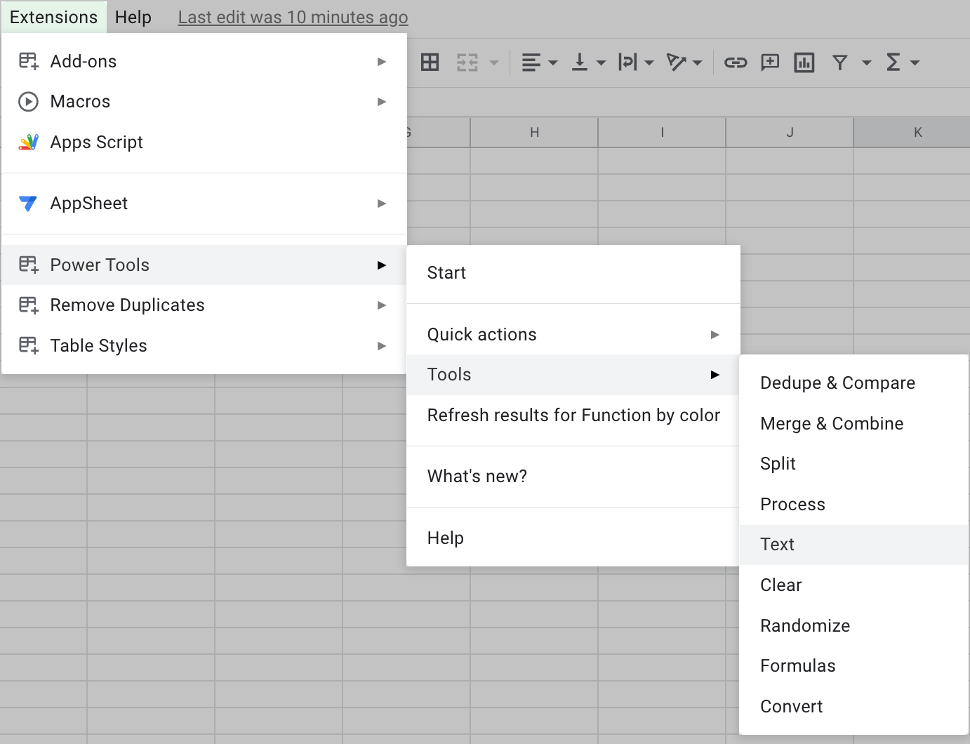
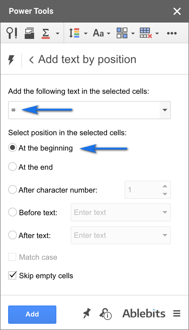
- Open Add text by position and add an equal sign (=) to add it at the beginning of each cell:
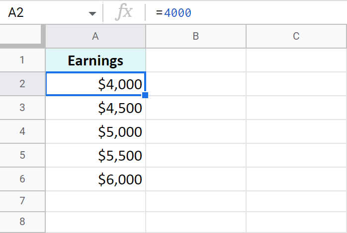
- Click Run to turn all your numbers to formulas:
- Proceed to the Formulas tool in Power Tools and select the option to modify all selected formulas.
You will see %formula% is already written there. You are to add those calculations you want to apply to all formulas at once.
Remember the formula to increase a number by percent?
=Amount*(1+%)Well, you already have those amounts in column A – this is your %formula% for the tool. Now you should only add the missing part to calculate the increase: *(1+10%). The whole entry looks like this:
%formula%*(1+10%)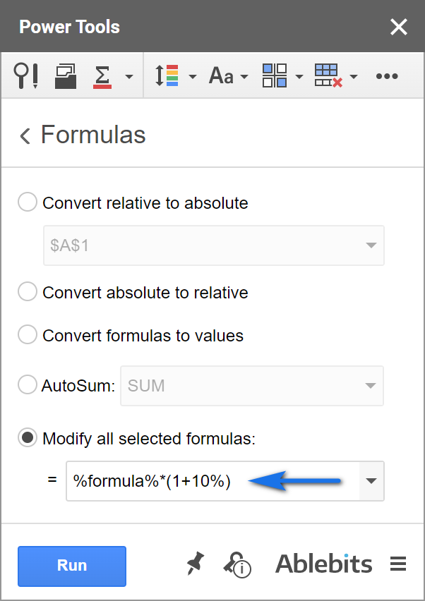
- Hit Run and all records will be raised by 10% at once:
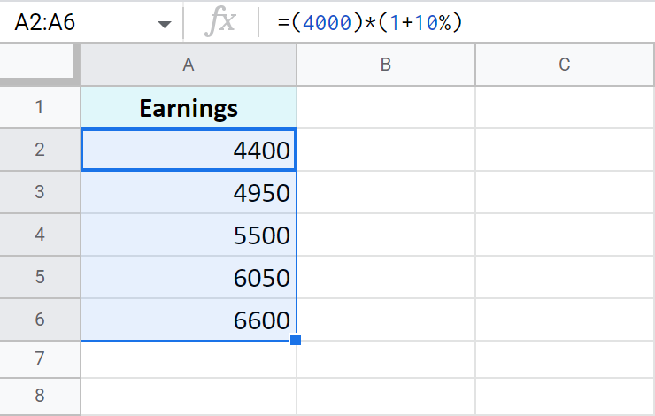
Tip. Feel free to apply any number format back to these formulas.
Click the button below to install Power Tools for Google Sheets and do the same with your data.
That's it! All these examples are easy-to-follow and are intended to remind those of you who've forgotten or show those who don't know the basic rules of calculating percentage in Google Sheets.
Spreadsheet with formula examples
Google Sheets percentage formulas (make yourself a copy to practice)
 by
by
198 comments
It helps a lot, thanks
Thank you for your feedback! We're glad the article helps!
Hello! This has been super informative! Thank you for your helpful article!
`
I have a situation which I haven't seen addressed anywhere, even in the diverse comments already here.
I would like to calculate a decaying percentage, but I can't figure out how to do it.
I'm looking to offer a 50%-per-person bundle discount, so Person A would be full price, but their friend, Person B, would be 50% the cost of person A, and Person A's other friend, Person C, would be 50% the cost of Person B, or 25% of the full price, etc. I can't figure out how to calculate this, though it doesn't seem impossible, given the following data points:
Column A = price for item (i.e. 100% of cost, what Person A would pay)
Column B = number of persons (variable)
Column C = adjusted price, decaying the percentage discount per person (so Person A would pay the full $8, say, and Person A+B would be $12, Persons A+B+C would be $14, etc.)
(I know this is a terrible business model, but I'm a teacher working out a fun sharing-is-caring incentive system for my classroom, so profit is not the goal. The "dollars" are not real anyway. haha)
Hello Nate,
Thank you for your feedback!
The answer to your question is explained in this section: Increase and decrease numbers by percentage
Assuming you have $8 in C2. In C3 you need a formula just like I provided in that section: =C2*(1-50%). It'll return 4 for the next person in C3. Then you just copy the formula down the column for as many rows as you need. And each row will return a number 50% less than the one above.
Thank you!!
So there's no more concise way to make this work? I was hoping for some insightful formula I could put into one cell to manage the calculation of decaying percentage.
Is there a way to have it calculate the final price based on the number in a "number of persons" cell?
Thank you so much for your help and super fast response, Natalia!!!
If you want to show the adjusted price per person with one formula, you can wrap everything in ArrayFormula while changing one-cell reference to the entire range, like this:
=ArrayFormula(C2:C10*(1-50%))
But you have to know the exact number of rows with people for it (10 in my example). If you'd rather make the formula check where the list of people in column B ends, the formula can look like this:
=ArrayFormula(IF(B3:B<>"",C2:C*(1-50%),""))
But this one will turn to error if you manually enter something somewhere in column C starting from C2. (Learn more about IF function in this article)
If you want one formula to return the last decreased price only (based on the count of people), use this one:
=100*POWER(0.5,COUNTA(B2:B)-1)
where 100 is the initial price; 0.5 is for 50% change; B2:B is your columns with names; and -1 for the first person with the initial price.
Hope this helps!
Thank you so much!!
This is very interesting and helpful!
It seems like there isn't a way to do what I'm hoping for.
I would like to streamline the process so there is no need to enter a list of names, but instead just type the number of friends into a cell, and have a formula present the final price, given the original price, for that number of friends. It seems like the second formula you shared would almost get there, but not quite...
Thank you again, Natalia! This has been very interesting and I'm learning so much.
-Nate
You're most welcome, Nate!
Formulas are super adjustable. If you know the number of people and want to simply enter this number into a cell, you won't need to count people, right? In this case, you just need to replace the count in the formula with the cell reference that contains that number – sounds logical, right? If so, here's the slight change you need to do if the number of people, say, in B2: =100*POWER(0.5,B2-1)
WOW!!! This is amazing, and it works perfectly!!!
I don't understand this new formula, but it does exactly what I was hoping for. This is much more complex than I had thought. I look forward to digging in and reading more about the ingredients you used to make this formula work, so I can make similar things myself in the future. What an impressive thing you have done, Natalia.
Thank you SO SO MUCH!!!
Nate
You're most most welcome, Nate! 😊
Hi again! I shared the sheet with you, with notes in some cells, to hopefully clarify how things "should" fit together, if I could have my way with things. haha
Most of the sheet is essentially *reference* for prices/options, and therefore irrelevant, for actually working on the formula. The formula and those parts of the layout it relies on are in the multi-color pink-outlined box in the upper right of each sheet.
Thank you SO SO MUCH for your help, Natalia!!!
Thank you for sharing the spreadsheet, Nate! Now your task is completely clear and I've found a formula for you – though it's not an easy one! 😅 I put it to J6 cell (the green one) on the Intended Outcome Sheet. Hope this is what you need! 😊
I guess I'll repeat it here as well in case someone is looking for a similar solution:
=H4 + SUM(SCAN(H4, MAKEARRAY(1, J4, LAMBDA(x, y, y)), LAMBDA(acc, y, acc * 0.5)))
where H4 - the price; J4 - the number of people; 0.5 - the desired percent change
Hi Natalia,
Thank you for this!! I have tried this formula, and I was initially confused, but I realize now that it seems to do exactly what you describe, instead of what I had hoped for. haha You did warn me that it would return the *last person's* portion of the price that would be needed, but I wonder if there is a way to have it output the full price, given a certain number of people.
So, I guess I'd need something that:
a) calculates the fraction of the cost corresponding to each person, and then
b) adds those fractions together, with the original price for the full cost at the "group rate".
I feel like I'm closer to seeing how that might happen, but it's not coming together just yet. Can you think of a way to pull off those two components in one formula, or perhaps with two cells with formulas that work together, maybe? Does there need to be one cell for step (a) and one for step (b)?
Hi Nate,
Could you please share a small sample spreadsheet with me (support@apps4gs.com)? Please include 2 sheets: (1) an example of your source data (2) the result you expect to get. The result sheet is of great importance as it usually gives a better understanding than any text description. I kindly ask you to shorten the tables to 10-20 rows.
Note. We keep that Google account for file sharing only and don't monitor its Inbox. Do not email there. Once you share the file, just confirm by replying to this comment.
I'll look into it and try to help :)
Good Afternoon, I am trying to get 10% of a total number in my Sheet and I cannot seem to find the correct formula for that. Please help!! Thank you!
Good afternoon, Andrea.
You will find formulas here: Percentage of a total in a Google spreadsheet
Hello, I want to calculate the percentage of sub processes progress and reflect the percentage to main process, noting that the sub processes and main process on different sheets can you please advice
Hello Yousef,
If I understand your task correctly, the examples from Percentage of a total will help you. You can easily reference cells from different sheets like this: =Sheet1!A1 or ='Sheet number two'!B4
I have a spreadsheet created to show cost of merchandise, I need the cost in one column, then add markups of 8% to those, and I want the new total in a new column. How can I get this to figure into the spreadsheet correctly so when I enter a number in Column D it automatically adds 8% and places that total in column E? Thanks
Hello Carlie,
You'll see formulas that add or subtract percent from numbers in this section: Increase and decrease numbers by percentage
I am attempting to calculate student grades that have improved from one test measure to the next. I have two columns (B and C) where I have recorded the two scores and I have set the formula to =percentif (B2:C32, "valueC>valueB") to see if I can calculate the percent of students who had an increase in score from test 1 to test 2. I keep getting a percent of 0 (even though I can see there are student who did in fact improve). Is there a better way to calculate a percent of students who have shown improvement between two test measures using two columns of the spreadsheet? Any help with what formula wording might work with this scenario is appreciated!
Hello Shayne,
The PERCENTIF function is not equipped to handle comparisons between two ranges in the way you're attempting. Instead, use this formula:
=COUNTIF(ARRAYFORMULA(C2:C32-B2:B32),">0")/COUNT(B2:B32)
COUNTIF calculates the number of students who improved their scores. COUNT calculates the total of students. And then divide one by another to find the percentage. Don't forget to apply the Percent format to the result.
Thank you so much! I appreciate the help. :-)
Shayne
You're welcome :)
Hello,
i have a 1k students and i need to know how many have a grade of 60% or higher and lower
what formula can i use?
thanks
Hi! To count the number of values by condition, use the COUNTIF function and these instructions: Google Spreadsheet COUNTIF function with formula examples.
thank you for your help!
hi, I'm not too savvy with formulas. I'm creating a spreadsheet on which teachers will enter an assessment score (whole number). That score is __/60; and I'd like the value in the cell to be represented as the percentage. Thanks in advance.
Hi! You can, in another cell, calculate the percentage using this whole number.
=A1/60
Set the percentage format in this cell. Read more: Percentage in Google Sheets - tutorial with useful formulas.
Next Question: How can I format a range of numbers to be a certain color? For example: scores between 0-69 in red, 70-79 in yellow, 80-100 in green, etc.
Hi,
You need to use conditional formatting to do that.
thank you so much!
You're most welcome, Kathy!
I am trying to figure out and "if equal to or less than "amount" multiply by 6.5% of cell value and if greater than "amount" multiply by 8.5% of cell value. example:
If cell F1 is equal to or less than $40,000, multiply the amount input into cell F1 by 6.5%, but if cell F1 is greater than $40000, multiply the amount input in cell F1 by 8.5%
Hello Daniel,
What you describe is what the IF function does. Check out this tutorial to learn how to build its formulas.
I'm trying to figure out how to set each cell in column B to calculate percentage from each adjoining cell in column A, using 1's for correct answer and 0's for incorrect answers, so looking for percentage of correct answers. Can you help please? Example below:
Column A Column B
10110001000 Need % from adjoining cell in column A
0011111001110 Need % from adjoining cell in column A
Hello Michael,
I'm sorry but your task is not clear. Please consider sharing an editable copy of your sample spreadsheet with us (support@apps4gs.com) and include the result you'd like to get. I kindly ask you to shorten the tables to 10-20 rows.
Note. We keep that Google account for file sharing only and don't monitor its Inbox. Please do not email there. Once you share the file, just confirm by replying to this comment.
I am looking to get percentages for individuals, the number of jobs they’ve done and the number of incidents.
Joe measured 10 jobs (B1 name)
Out of 10 jobs (using check box) 5 had incidents (C1 check box)
Joe has a 50% incident rate (D1 percentage)
I hope I am asking this question accurately
Hello Zac,
Have you tried this formula? If it doesn't work as you need, please consider sharing an editable copy of your sample spreadsheet with us (support@apps4gs.com) and include the result you'd like to get & your formula.
Note. We keep that Google account for file sharing only and don't monitor its Inbox. Please do not email there. Once you share the file, just confirm by replying to this comment.
Hello! I have a bit of a complicated one. Is there a way to have a formula that can calculate a score based on certain criteria being checked off?
A3: Drop Down Menu (option A - 0%, option B - 10%, option C - 20%, option D - 30%)
B3: Check Box - 20% if checked
C3: Check Box - 20% if checked
D3: Check Box - 5% if checked
E3: Check Box - 25% if checked
F3: total score
the criteria being if the drop down menu has option D selected, and all boxes checked, that would be a score of 100%. Then of course, the score would change depending on what is checked or which drop down option applies.
So is there a formula that can do this? I know it's a little complicated!!
Hello Sarah,
If I understand your task correctly, the solution I offered below to Jeanne will help you as well. You just need to replace ">0" with TRUE (for checked items).
How would I calculate this--
What percentage of the values in this column are less than ________?
Hello Anne-Marie,
Please see my reply to Jeanne below, it's the same task and I offered the solution.
Hi, I'm a little stuck and hoping you can help. Lets say in column A I have a list of names (person 1, person 2, person 3, person 1, person 2, person 3) which appear multiple times and not in the same order, and Column B states YES or NO next to each name. How can I calculate the percentage of YES or NO for each person if the names appear multiple times in Column A? Thanks!
Hi Rebecca,
To find percentage of a total, you need to divide the number by total.
The total here is all occurrences of each name: =COUNTIF(A2:A10,A2)
Where A2 is person 1.
The amount of YES next to person 1:
=COUNTIFS(A2:A10,A2,B2:B10,"yes")
The percentage of YES:
=COUNTIFS(A2:A10,A2,B2:B10,"yes")/COUNTIF(A2:A10,A2)
You count all NO for person 1 in a similar manner.
To count this for other people, change A2 accordingly.
Functions used in the formula:
COUNTIF
COUNTIFS
Thanks SO much for the fast response. This is exactly what I needed!
You're most welcome, Rebecca, glad I could help! :)
I have a column of numbers. I'd like to be able to find out the percentage of how many times the numbers in this list are greater than 0.
Example:
0
0
4
-1
This would be 25%.
Is there a formula for this?
Hello Jeanne,
Yes, here you go (assuming these values are in B2:B5):
=COUNTIF(B2:B5,">0")/COUNT(B2:B5)
Apply the Percent format to the resulting cell as described in this part of the article.
Functions in use:
COUNTIF
COUNT
I need to make a column of percentages based on a column of fractions. So my column C has fractions (example: 20/43) and I want column D to show thoses in percentages.
Hello Elizabeth,
If I understand your task correctly, you should be able to calculate that by following the steps in this part of the article.
Hello, I would like to capture the percentage of three numbers (represents three year totals) to see a trend either negative or positive.
Thank you,
Brian
Hello Brian,
For me to be able to help you, please describe the task in detail. Provide examples of the data you have and specify how you want it to look as a result. Thank you.
Hello,
I am working with year-to-date statistics over a three-year period covering 2021, 2022, 2023. Example: 2021= 40 2022= 45 and 2023= 35. I would like to reflect a positive or negative % over the three year period. I used this function =TO_PERCENT((Q29-Z27)/Z27) to calculate 2022 and 2023 and it reports -22% which is perfect. Except I need it for three years, I’m not sure how to include 40 from 2021 into the equation. The total for 2021 is displayed in H29 with the percentage result being displayed on the same sheet in Z29
Your expertise is certainly appreciated by many.
Hello Brian,
Thank you for the details. So you need to calculate the percent change between 2023 and 2021, correct?
Hello,
Correct, showing a % trend. Is 2023 higher or lower than 2021 & 2022
Thank you again.
If you're trying to compare 2023 with 2021 & 2022, you will need 2 formulas:
If you need both results in the same cell, you will have to concatenate the calculations:
=ROUND((B4-B3)/B3*100)&" & "&ROUND(((B4-B2)/B2)*100)
If I'm missing something and this is not what you want, please specify the result you expect to get. Thanks!
Hi,
I was wondering if you can make a progress bar, once a certain numbers of cells are checked pr have a certain color.
Thank you
Hi Marian,
You can try a way I suggested earlier to Darsha
Hi,
I need to figure out the following.
Example:
I need the total from row 1 plus the total from row 2 plus just 30% of the total from row 3, how would this be done?
Thanks
Hi John,
You can use the SUM function. To find 30% of the total from one row correctly, use this method.
Hi Natalia,
I've already learned a bunch through your posts so please keep it up!!
I do have a question i can't seem to find the answer to though, if you could point me in the right direction i'd be forever grateful to you!
I'm building out a material spreadsheet for my plumbing company, I have a cell that is designated for my cost from supplier. My material markup is based on a sliding range meaning the higher the cost, the less my markup percentage will be.
For example,
from $.01-$5 the markup will be 4x
from $5.01-$10 the markup will be 3.25x
and so on...
Is there a way to set up a few different formulas based on different cost ranges and different percentages to calculate my selling price? This spread sheet is roughly 1400 items and my cost gets updated once every two months so going through each line item would take forever.
If you have any insight on how to do this or what you feel would be the best way to go about it i'd greatly appreciate it.
Thank you!
Hi Devin,
If I understand your task correctly, you need to use the IF function. It will check the cost and calculate the percentage accordingly.