This tutorial shows how to make an Excel formula for percent increase or decrease and use it with both positive and negative numbers.
In Microsoft Excel, there are 6 different functions for calculating variance. However, none of them is suitable for calculating the percent difference between two cells. The inbuilt functions are designed to find variance in the classical sense, i.e. how far a set of values are spread out from their average. A percent variance is something different. In this article, you will find the right formula for calculating percent change in Excel.
What is percentage change?
Percent change, aka percentage variance or difference, is a proportional change between two values, an original value and a new value.
Percent change formula calculates how much something changes between two periods percentage-wise. For example, you can calculate variance between sales in this year and last year, between a forecast and observed temperature, between a budgeted cost and the real one.
For instance, in January you earned $1,000 and in February $1,200, so the difference is a $200 increase in earnings. But how much is that in terms of percentage? To find that out, you use a percent change formula.
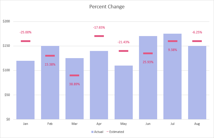
Excel percent change formula
There are two basic formulas to find the percentage difference between two numbers.
Classic percentage variance formula
Here is the generally used formula to calculate the percent change:
In math, you'd normally perform 3 steps to calculate the percentage variance between any two numeric values:
- Subtract the new value from the old one.
- Divide the difference by the old number.
- Multiply the result by 100.
In Excel, you skip the last step by applying the Percentage format.
Excel percent change formula
And here is a simpler formula for percentage change in Excel that returns the same result.
How to calculate percent change in Excel
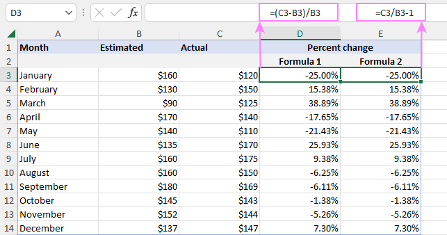
To find the percentage difference between two numbers in Excel, you can use either of the above formulas. Let's say you have the estimated sales in column B and actual sales in column C. Assuming the estimated number is the "baseline" value and actual is the "new" value, the formulas take this shape:
=(C3-B3)/B3
or
=C3/B3-1
The above formulas compare the numbers in row 3. To calculate the percent of change in the entire column, this is what you need to do:
- Enter the percent difference formula in any blank cell in row 3, say in D3 or E3.
- With the formula cell selected, click the Percent Style button on the ribbon or press the Ctrl + Shift + % shortcut. This will convert the returned decimal number to percentage.
- Drag the formula down across as many rows as needed.
After copying down the formula, you'll get a percent change column from your data.
How Excel percent change formula works
When doing the calculations manually, you would take an old (original) value and a new value, find the difference between them and divide it by the original value. To get the result as percentage, you would multiply it by 100.
For example, if the initial value is 120 and the new value is 150, the percent difference can be calculated in this way:
=(150-120)/120
=30/120
=0.25
0.25*100 = 25%
Applying the Percentage number format in Excel displays a decimal number as percentage automatically, therefore the *100 part is omitted.
Excel formula for percent increase /decrease
As percent increase or decrease is just a particular case of percentage variance, it is calculated with the same formula:
Or
For example, to calculate the percent increase between two values (B2 and C2), the formula is:
=(C2-B2)/B2
Or
=C2/B2-1
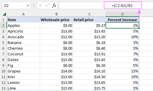
A formula to calculate the percent decrease is exactly the same.
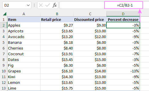
Excel percent change absolute value
By default, the percentage variance formula in Excel returns a positive value for percent increase and a negative value for percent decrease. To get the percentage change as an absolute value without regard to its sign, wrap the formula in the ABS function like this:
In our case, the formula takes this form:
=ABS((C3-B3)/B3)
This one will also work fine:
=ABS(C3/B3-1)

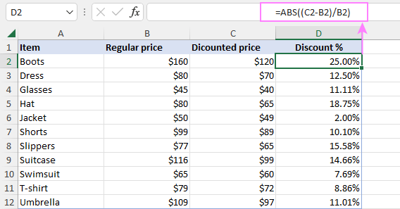
Calculate discount percentage
This example shows one more practical use of the Excel percent change formula - working out a discount percentage. So, ladies, when you go shopping, remember this:
discount % = (discounted price - regular price) / regular price
discount % = discounted price / regular price - 1
A discount percent is displayed as a negative value because the new discounted price is smaller than the initial price. To output the result as a positive number, nest formulas inside the ABS function like we did in the previous example:
=ABS((C2-B2)/B2)
Calculate the value after percent change
To get a value after the percentage increase or decrease, the generic formula is:
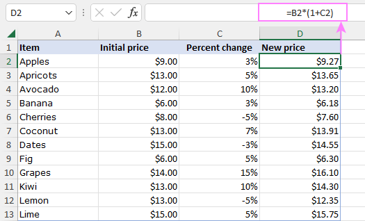
Suppose you have the original values in column B and the percentage difference in column C. To compute the new value after the percentage change, the formula in D2 copied down is:
=B2*(1+C2)
First, you find the overall percentage that needs to be multiplied with the original value. For this, just add the percent to 1 (1+C2). And then, you multiply the overall percentage by the original numbers to get the desired result.
As you can see, this solution works nicely for both percentage increase and decrease:
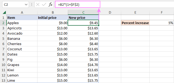
To increase or decrease an entire column by a certain percent, you can supply the percentage value directly in a formula. Say, to increment all the values in column B by 5%, enter the below formula in C2, and then drag it down across the remaining rows:
=B2*(1+5%)
Here, you simply multiply the original value by 105%, which produces a value that is 5% higher.
For convenience, you can input the percentage value in a predefined cell (F2) and refer to that cell. The trick is locking the cell reference with $ sign, so the formula copies correctly:
=B2*(1+$F$2)
The advantage of this approach is that to increase a column by another percentage, you only need to change the value in a single cell. Since all the formulas are linked to that cell, they will recalculate automatically.
Calculating percent variance with negative values
If some of your values are represented by negative numbers, the traditional percent difference formula will work incorrectly. A commonly accepted solution is to make the denominator a positive number with the help of the ABS function.
Here's a generic Excel formula for percent change with negative numbers:
With the old value in B2 and the new value in C2, the real formula goes as follows:
=(C2-B2)/ABS(B2)
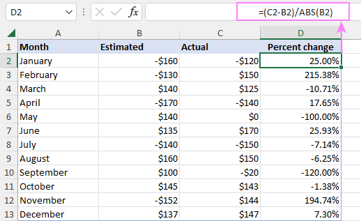
Note. Although this ABS adjustment is technically correct, the formula may produce misleading results in case the original value is negative and new value is positive, and vice versa.
Excel percent change divide by zero error (#DIV/0)
If your data set contains zero values, you are likely to run into a divide by zero error (#DIV/0!) when calculating percentage change in Excel because you cannot divide a number by zero in math. The IFERROR function can help to overcome this problem. Depending on your expectations for the final result, use one of the following solutions.
Solution 1: if the old value is zero, return 0
If the old value is zero, the percentage change would be 0% regardless of whether the new value is zero or not.
=IFERROR((C2-B2)/B2, 0)
or
=IFERROR(C2/B2-1, 0)
Solution 2: if the old value is zero, return 100%
This solution implements another approach assuming that the new value has grown by 100% starting from zero:
=IFERROR((C2-B2)/B2, 1)
=IFERROR(C2/B2-1, 1)
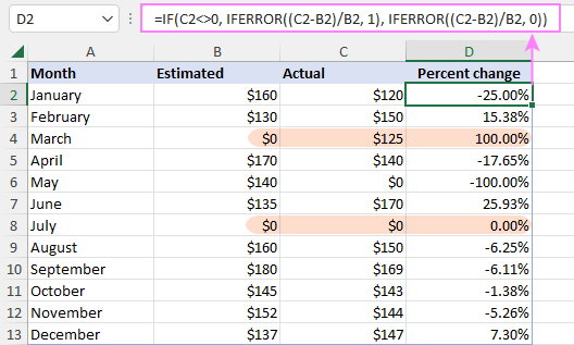
In this case, the percent difference would be 100% if the old value is zero (row 5) or both values are zeros (row 9).
Looking at the highlighted records below, it becomes evident that neither formula is perfect:

To get better results, you can combine the two formulas into one using the nested IF statement:
=IF(C2<>0, IFERROR((C2-B2)/B2, 1), IFERROR((C2-B2)/B2, 0))
This improved formula will return:
- The percent change as 0% if both the old and new values are zeros.
- The percent change as 100% if the old value is zero and the new value is not zero.
That's how to calculate a percent increase or decrease in Excel. For hands-on experience, you are welcome to download our sample workbook below. I thank you for reading and hope to see you on our blog next week!
Practice workbook for download
Excel formula for percent increase /decrease - examples (.xlsx file)
 by
by
10 comments
Some of my customers want me to include my management fee as part of their total ad spend. For example they have an annual budget of $10,000 which they want me to include my 15% management fee. Through trial and error I've determined that the ad spend should be $8,695.66 plus a 15% ($1,304.34) management fee for a total of $10,000,
Is there a function or way in Excel to find the $1,304.34 value without the trial and error?
Hi!
If I understood you correctly, the following formula is studied at school:
=10000*15/115
I am trying to generate a variance between a negative point and then a positive point (i.e. -400 in year 1 to 100 in year 2). In the scenario above, the result should produce a positive % variance, however, I cannot seem to find a good number applying traditional formulas like you have above. I've been looking at a lot forums and different opinions, but I cannot seem to get a one answer. Please let me know if you have any information that might be able to help me.
Hello!
To calculate the percent deviation with negative numbers, use the ABS function:
=(C3-B3)/ABS(B3)%
am calculating cost variance.
budget 500 and actual 400 - 20%
budget 400 and actual 500 25%
Why the same amount giving two different percentages?
The equations are calculating the % movement from different baselines, hence the actual movement amount provides a different %. Try the same with:
Budget 100 and actual 90
Budget 90 and actual 100
if it helps with the logic.
How do I do V look up
Hi Philip,
You'll find a detailed explanation in this tutorial: Excel VLOOKUP tutorial with formula examples
Formula for calculating year-on-year % variations:
IF(ISERROR((D4/C4)-1);"n.a.";IF(((D4/C4)-1)>1;">100.0%";IF(((D4/C4)-1)<-1;"<-100.0%";((D4/C4)-1))))
This formula does not work when old value is 0 and new value is not 0. It shows "n.a" instead of 100%. Use "=IF(D40, IFERROR((D4-C4)/C4, 1), IFERROR((D4-C4)/C4, 0))"